Data Science different topic's explanation -- Part-10 -- Discrete distributions

[anish-arya]

This is data science different topic explanation conversation series.
If you are not following below mentioned are the links for each part.

Part-1:

Data Science different explanation -- An introduction

Data Science different explanation – An introduction [image] There are a lot of engineers who have never been involved in the field of statistics or Data Science. But in order to build data pipelines or rewrite produced code by Data Scientists to an adequate, easily maintained code many nuances and misunderstandings arise on the engineering side. For those Data/ML engineers and novice Data Scientists, I’ve made this series of posts. I will try to explain some basic approaches in plain eng…

Part-2:

Data Science different topic explanation -- Part-2 -- Events. Probabilities of events

If you missed the previous post, here’s the below mentioned link. Data Science different topic explanation – Part-2 – Events. Probabilities of events One of the basic concepts in statistics in an event. Events are simply results of experiments. Events can be certain impossible, or random. A certain event is an event that as a result of an experiment (the execution of certain actions with a certain set of conditions) will occur in 100% cases. For instance, tossed coin will certainly fall (on…

Part-3:

Data Science different topic explanation -- Part-3 -- Event Types

This is Data Science different topic explanation conversation series. If you are not following this conversation series below are the link: Part-1: Part-2: Data Science different topic explanation – Part-3 – Event Types Independent and Dependent events Two random events A and B are called independent if the occurrence of one of them does not change the probability of the occurrence of the other. Otherwise, events A and B are called dependent. Counterintuitively, knowing that the coin l…

Part-4:

Data Science different topic explanation -- Part-4 -- Disjoint and overlapping events

This is data science different topic explanation conversation series. If you are not following below mentioned are the links for each part. Part-1: Part-2: Part-3: Data Science different topic explanation – Part-4 – Disjoint and overlapping events Disjoint events cannot happen at the same time. A synonym for this term is “mutually exclusive”. For instance, the outcome of a single coin toss cannot be head and a tail, it can be either head or tails. The not disjoint event can happend a…

Part-5:

Data Science different topic's explanation -- Part-5 -- Types of Probabilities

This is data science different topic explanation conversation series. If you are not following below mentioned are the links for each part. Part-1: Part-2: Part-3: Part-4: Data Science different topic’s explanation – Part-5 – Types of Probabilities Joint Probability Joint probability is a type of probability where more than one event can occur simultaneously. The joint probability is the probability that event A will occur at the same time as event B. For instance, from a deck o…

Part-6:

Data Science different topic's explanation -- Part-6 -- Marginal Probability and Conditional Probability

This is data science different topic explanation conversation series. If you are not following below mentioned are the links for each part. Part-1: Part-2: Part-3: Part-4: Part-5: Data Science different topic’s explanation – Part-6 – Marginal Probability and Conditional Probability Marginal Probability Marginal Probability – a probability of any single event occurring unconditioned on any other events. Whenever someone asks you whether the weather is going to be rainy or sunny t…

Part-7:

Data Science different topic's explanation -- Part-7 -- Probability Distributions

Continuing the conversation series for next topic here. Cumulative Distribution Function (CDF) The cumulative distribution function provides an integral picture of the probability distribution. As the name cumulative suggests, it is simply the probability that a variable will take a value less than or equal to particular value. In the example above given x=3, the CDF tells us the sum probability of all random variables form 1 to 3.

Part-8:

Data Science different topic's explanation -- Part-8 -- Continuous distributions

This is data science different topic explanation conversation series. If you are not following below mentioned are the links for each part. Part-1: Part-2: Part-3: Part-4: Part-5: Part-6: Part-7: Continuous distributions We investigate probabilistic distributions of continuous random variables, i.e. random variables whose support contains an infinite range of possible outcomes. Uniform Distribution A uniform distribution is a type of distribution of probabilities where all …

Part-9:

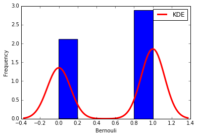
Data Science different topic's explanation -- Part-9 -- Normal Distribution

This is data science different topic explanation conversation series. If you are not following below mentioned are the links for each part. Part-1: Part-2: Part-3: Part-4: Part-5: Part-6: Part-7: Part-8: Data Science different topic’s explanation – Part-9 – Normal Distribution from scipy.stats import norm import matplotlib.pyplot as plt import numpy as np def normal() -> None: fig, ax = plt.subplots(1, 1) # calculate a few first moments mean, var, skew, kurt = n…

Data Science different topic’s explanation – Part-10 – Discrete distributions

Bernoulli distribution (binomial distribution)

from scipy.stats import bernoulli
import seaborn as sb


def bernoulli_dist(): -> None:
    data_bern = bernoulli.rvs(size=1000,p=0.6)
    ax = sb.distplot(
        data_bern, 
        kde=True, 
        color='b', 
        hist_kws={'alpha':1},
        kde_kws={'color': 'r', 'lw': 3, 'label': 'KDE'})
    ax.set(xlabel='Bernouli', ylabel='Frequency')

bernoulli_dist()

Not all phenomena are measured on a quantitative scale of type 1,2,3 … 100500… Not always a phenomenon can take on an infinite or a large number of different states. For instance, a person’s sex can be either a man or a woman. The shooter either hits the target or missed. You can vote either “for” or “against”, etc. Other words reflect the state of an alternative feature (the event did not come).

[anish-arya]

Continuing the left out content here of above post.

The upcoming event (positive outcome) is also called “success”. Such phenomena can also be massive and random. Therefore, they can be measured and make statistically valid conclusions.

Experiment with such data are called the Bernoulli scheme, in honor of the famous Swiss mathematician, who found that with a large number of tests, the ratio of positive outcomes to the total number of tests converges to the probability of the occurrence of this event.

[anish-arya]

Continuing the missed out content here.

• n – the number of experiments in the series;
• x – a random variable (the number of occurrences of the event);
• Px – the probability that event happens exactly x times;
• q = 1 - p (the probability that the event does not appear in the test)