The error function that we have considered to optimize is relatively simple, because it is convex and characterised by a single global minimum.
Nonetheless, in the context of machine learning, we often need to optimize more complex functions that can make the optimization task very challenging. Optimization can become even more challenging if the input to the function is also multidimensional.
Calculus provides us with the necessary tools to address both challenges.
Suppose that we have a more generic function that we wish to minimize, and which takes a real input, x, to produce a real output, y:
y = f(x)
Computing the rate of change at different values of x is useful because it gives us an indication of the changes that we need to apply to x, in order to obtain the corresponding changes in y.
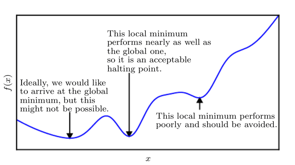
Since we are minimizing the function, our goal is to reach a point that obtains as low a value of f(x) as possible that is also characterised by zero rate of change; hence, a global minimum. Depending on the complexity of the function, this may not necessarily be possible since there may be many local minima or saddle points that the optimisation algorithm may remain caught into.
In the context of deep learning, we optimize functions that may have many local minima that are not optimal, and many saddle points surrounded by very flat regions.
Page 84, Deep Learning, 2017.
Hence, within the context of deep learning, we often accept a suboptimal solution that may not necessarily correspond to a global minimum, so long as it corresponds to a very low value of f(x).
Line Plot of Cost Function to Minimize Displaying Local and Global Minima
Taken from Deep Learning
If the function we are working with takes multiple inputs, calculus also provides us with the concept of partial derivatives; or in simpler terms, a method to calculate the rate of change of y with respect to changes in each one of the inputs, x i, while holding the remaining inputs constant.
This is why each of the weights is updated independently in the gradient descent algorithm: the weight update rule is dependent on the partial derivative of the SSE for each weight, and because there is a different partial derivative for each weight, there is a separate weight update rule for each weight.
Page 200, Deep Learning, 2019.
Hence, if we consider again the minimization of an error function, calculating the partial derivative for the error with respect to each specific weight permits that each weight is updated independently of the others.
This also means that the gradient descent algorithm may not follow a straight path down the error surface. Rather, each weight will be updated in proportion to the local gradient of the error curve. Hence, one weight may be updated by a larger amount than another, as much as needed for the gradient descent algorithm to reach the function minimum.


 SQL
SQL
 HTML/CSS/JS
 Coding


 Settings
 Logout