Time series forecasting is a difficult problem with no easy answer. There are countless statistical models that claim to outperform each other, yet it is never clear which model is best.
That being said, ARMA-based models are often a good model to start with. They can achieve decent scores on most time-series problems and are well-suited as a baseline model in any time series problem.
Introduction
The ARIMA model acronym stands for “Auto-Regressive Integrated Moving Average” and for this article we will will break it down into AR, I, and MA.
Autoregressive Component — AR(p)
The autoregressive component of the ARIMA model is represented by AR(p), with the p parameter determining the number of lagged series that we use.

AR(0): White Noise
If we set the p parameter as zero (AR(0)), with no autoregressive terms. This time series is just white noise. Each data point is sampled from a distribution with a mean of 0 and a variance of sigma-squared. This results in a sequence of random numbers that can’t be predicted. This is really useful as it can serve as a null hypothesis, and protect our analyses from accepting false-positive patterns.
AR(1): Random Walks and Oscillations
With the p parameter set to 1, we are taking into account the previous timestamp adjusted by a multiplier, and then adding white noise. If the multiplier is 0 then we get white noise, and if the multiplier is 1 we get a random walk. If the multiplier is between 0 < α₁ < 1, then the time series will exhibit mean reversion. This means that the values tend to hover around 0 and revert to the mean after regressing from it.
AR(p): Higher-order terms
Increasing the p parameter even further is just means going further back and adding more timestamps adjusted by their own multipliers. We can go as far back as we want, but as we get further back it is more likely that we should use additional parameters such as the moving average (MA(q)).
Moving Average — MA(q)
“This component is not a rolling average, but rather the lags in the white noise.” — Matt Sosna
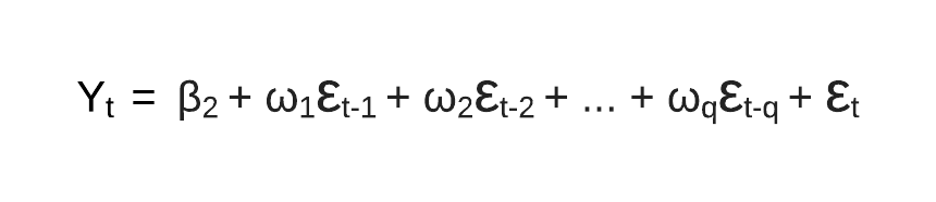
MA(q)
MA(q) is the moving average model and q is the number of lagged forecasting error terms in the prediction. In an MA(1) model, our forecast is a constant term plus the previous white noise term times a multiplier, added with the current white noise term. This is just simple probability + statistics, as we are adjusting our forecast based on previous white noise terms.
ARMA and ARIMA Models
ARMA and ARIMA architectures are just the AR (Autoregressive) and MA (Moving Average) components put together.
ARMA
The ARMA model is a constant plus the sum of AR lags and their multipliers, plus the sum of the MA lags and their multipliers plus white noise. This equation is the basis of all the models that come next and is a framework for many forecasting models across different domains.
ARIMA
ARIMA Formula — By Author
The ARIMA model is an ARMA model yet with a preprocessing step included in the model that we represent using I(d). I(d) is the difference order, which is the number of transformations needed to make the data stationary. So, an ARIMA model is simply an ARMA model on the differenced time series.