Support Vector Machine Classification in Scikit-learn
Support Vector Machines
Generally, Support Vector Machines considered to be a classification approach but, it can be employed in both types of classification and regression problems. It can easily handle multiple continuous and categorical variables. SVM constructs hyperplane in multidimensional space to separate different classes. SVM generates optimal hyperplane in an iterative manner, which is used to minimize an error. The core idea of SVM is to find a maximum marginal hyperplane(MMH) that best divides the dataset into classes.

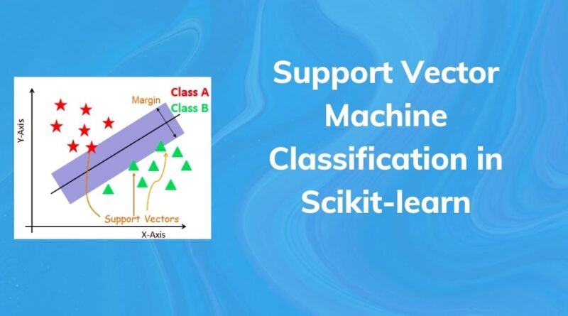
Support Vectors
Support vectors are the data points, which are closest to the hyperplane. These points will define the separating line better by calculating margins. These points are more relevant to the construction of the classifier.
Hyperplane
A hyperplane is a decision plane that separates between a set of objects having different class memberships.
Margin
A margin is a gap between the two lines on the closest class points. This is calculated as the perpendicular distance from the line to support vectors or closest points. If the margin is larger in between the classes than it is considered as good margin otherwise it is a bad margin.
How does SVM work?
The main objective is to segregate the given dataset in the best possible way. The distance between the nearest points is known as the margin. The objective is to select a hyperplane with the maximum possible margin between support vectors in the given dataset. SVM searches for the maximum marginal hyperplane in the following steps:
-
Generate hyperplanes that segregate the classes in a better way. Left-hand side figure showing three hyperplanes black, blue, and orange. Here, the blue and orange have higher classification errors, but the black is separating the two classes correctly.
-
Select the right hyperplane with the maximum segregation from either nearest data points as shown in the right-hand side figure.

Dealing with non-linear and inseparable planes
Some problems can’t be solved using linear hyperplane, as shown in the figure below (left-hand side).

In such a situation, SVM uses a kernel trick to transform the input space to a higher dimensional space as shown on the right. The data points are plotted on the x-axis and z-axis (Z is the squared sum of both x and y: z=x²=y²). Now you can easily segregate these points using linear separation.
SVM Kernels
The SVM algorithm is implemented in practice using a kernel. A kernel transforms an input data space into the required form. SVM uses a technique called the kernel trick. Here, the kernel takes a low-dimensional input space and transforms it into a higher-dimensional space. In other words, you can say that it converts non-separable problems to separable problems by adding more dimension to it. It is most useful in a non-linear separation problem. Kernel trick helps us to build a more accurate classifier.
- Linear Kernel A linear kernel can be used as a normal dot product any two given observations. The product between two vectors is the sum of the multiplication of each pair of input values.
K(x, xi) = sum(x * xi)
- Polynomial Kernel A polynomial kernel is a more generalized form of the linear kernel. The polynomial kernel can distinguish curved or nonlinear input space.
K(x,xi) = 1 + sum(x * xi)^d
Where d is the degree of the polynomial. d=1 is similar to the linear transformation. The degree needs to be manually specified in the learning algorithm.
- Radial Basis Function Kernel The Radial basis function kernel is a popular kernel function commonly used in support vector machine classification. RBF can map an input space in infinite-dimensional space.
K(x,xi) = exp(-gamma * sum((x – xi)^2)
Here gamma is a parameter, which ranges from 0 to 1. A higher value of gamma will perfectly fit the training dataset, which causes over-fitting. Gamma=0.1 is considered to be a good default value. The value of gamma needs to be manually specified in the learning algorithm.
Classifier Building in Scikit-learn
Till now, you have learned about the theoretical background of SVM. Now you will learn about its implementation in Python using scikit-learn.
In the model the building part, you can use the cancer dataset, which is a very famous multi-class classification problem. This dataset is computed from a digitized image of a fine needle aspirate (FNA) of a breast mass. They describe the characteristics of the cell nuclei present in the image.
The dataset comprises 30 features (mean radius, mean texture, mean perimeter, mean area, mean smoothness, mean compactness, mean concavity, mean concave points, mean symmetry, mean fractal dimension, radius error, texture error, perimeter error, area error, smoothness error, compactness error, concavity error, concave points error, symmetry error, fractal dimension error, worst radius, worst texture, worst perimeter, worst area, worst smoothness, worst compactness, worst concavity, worst concave points, worst symmetry, and worst fractal dimension) and a target (a type of cancer).
This data has two types of cancer classes: malignant (harmful) and benign (not harmful). Here, you can build a model to classify the type of cancer. The dataset is available in the scikit-learn library or you can also download it from the UCI Machine Learning Library.
Loading Data
Let’s first load the required dataset you will use.
#Import scikit-learn dataset library
from sklearn import datasets

#Load dataset
cancer = datasets.load_breast_cancer()
Exploring Data
After you have loaded the dataset, you might want to know a little bit more about it. You can check features and target names.
# print the names of the 13 features
print("Features: ", cancer.feature_names)

# print the label type of cancer('malignant' 'benign')
print("Labels: ", cancer.target_names)
Output: Features: [‘mean radius’ ‘mean texture’ ‘mean perimeter’ ‘mean area’ ‘mean smoothness’ ‘mean compactness’ ‘mean concavity’ ‘mean concave points’ ‘mean symmetry’ ‘mean fractal dimension’ ‘radius error’ ‘texture error’ ‘perimeter error’ ‘area error’ ‘smoothness error’ ‘compactness error’ ‘concavity error’ ‘concave points error’ ‘symmetry error’ ‘fractal dimension error’ ‘worst radius’ ‘worst texture’ ‘worst perimeter’ ‘worst area’ ‘worst smoothness’ ‘worst compactness’ ‘worst concavity’ ‘worst concave points’ ‘worst symmetry’ ‘worst fractal dimension’] Labels: [‘malignant’ ‘benign’]
Let’s explore it for a bit more. you can also check the shape of the dataset using shape.
# print data(feature)shape
cancer.data.shape
Output: (569, 30)
Let’s check the top 5 records of the feature set.
# print the cancer data features (top 5 records)
print(cancer.data[0:2])
Output: [[1.799e+01 1.038e+01 1.228e+02 1.001e+03 1.184e-01 2.776e-01 3.001e-01 1.471e-01 2.419e-01 7.871e-02 1.095e+00 9.053e-01 8.589e+00 1.534e+02 6.399e-03 4.904e-02 5.373e-02 1.587e-02 3.003e-02 6.193e-03 2.538e+01 1.733e+01 1.846e+02 2.019e+03 1.622e-01 6.656e-01 7.119e-01 2.654e-01 4.601e-01 1.189e-01] [2.057e+01 1.777e+01 1.329e+02 1.326e+03 8.474e-02 7.864e-02 8.690e-02 7.017e-02 1.812e-01 5.667e-02 5.435e-01 7.339e-01 3.398e+00 7.408e+01 5.225e-03 1.308e-02 1.860e-02 1.340e-02 1.389e-02 3.532e-03 2.499e+01 2.341e+01 1.588e+02 1.956e+03 1.238e-01 1.866e-01 2.416e-01 1.860e-01 2.750e-01 8.902e-02]]
Let’s check the records of the target set.
# print the cancer labels (0:malignant, 1:benign)
print(cancer.target[0:20])
Output: [0 0 0 0 0 0 0 0 0 0 0 0 0 0 0 0 0 0 0 1]
Splitting Data
To understand model performance, dividing the dataset into a training set and a test set is a good strategy.
Let’s split dataset by using function train_test_split(). you need to pass basically 3 parameters features, target, and test_set size. Additionally, you can use random_state to select records randomly.
# Import train_test_split function
from sklearn.model_selection import train_test_split

# Split the dataset into the training set and test set
X_train, X_test, y_train, y_test = train_test_split(cancer.data, cancer.target, test_size=0.3,random_state=109) # 70% training and 30% test
Generating Model
Let’s build a support vector machine model. First, import the SVM module and create a support vector classifier object by passing the argument kernel as the linear kernel in SVC() function.
Then, fit your model on the train set using fit() and perform prediction on the test set using predict().
#Import svm model
from sklearn import svm

#Create a svm Classifier
clf = svm.SVC(kernel='linear') # Linear Kernel

#Train the model using the training sets
clf.fit(X_train, y_train)

#Predict the response for test dataset
y_pred = clf.predict(X_test)
Evaluating the Model
Let’s estimate, how accurately the classifier or model can predict the breast cancer of patients.
Accuracy can be computed by comparing actual test set values and predicted values.
#Import scikit-learn metrics module for accuracy calculation
from sklearn import metrics

# Model Accuracy: how often is the classifier correct?
print("Accuracy:",metrics.accuracy_score(y_test, y_pred))
Output: Accuracy: 0.9649122807017544
Well, you got a classification rate of 96.49%, considered as very good accuracy.
For further evaluation, you can also check the precision and recall of the model.
# Model Precision: what percentage of positive tuples are labeled as such?
print("Precision:",metrics.precision_score(y_test, y_pred))

# Model Recall: what percentage of positive tuples are labeled as such?
print("Recall:",metrics.recall_score(y_test, y_pred))
Output: Precision: 0.9811320754716981 Recall: 0.9629629629629629
Well, you got precision 98% and recall 96%, considered as very good precision and recall value.
Tuning Hyperparameters
- Kernel: The main function of the kernel is to transform the given dataset input data into the required form. There are various types of functions such as linear, polynomial, and radial basis function (RBF). Polynomial and RBF are useful for non-linear hyperplane. Polynomial and RBF kernels compute the separation line in the higher dimension. In some of the applications, it is suggested to use the more complex kernel to separate the classes that are curved or nonlinear. This transformation can lead to more accurate classifiers.
- Regularization: Regularization parameter in python’s Scikit-learn C parameter used to maintain regularization. Here C is the penalty parameter, which represents misclassification or error term. Misclassification or error term tells the SVM optimization how much error is bearable. This is how you can control the trade-off between decision boundary and misclassification terms. The smaller value of C causes a small-margin hyperplane and a large value of C causes a larger-margin hyperplane.
- Gamma: The lower value of Gamma loosely fit the training dataset whereas the higher value of gamma will exactly fit the training dataset, which causes over-fitting. In other words, you can say the low value of gamma considers only nearby points in the calculation separation line whereas the high value of gamma considers all the points in the calculation of separation line.
Advantages
SVM Classifiers offer good accuracy and perform faster prediction compared to the Naïve Bayes algorithm. They also use less memory because they use a subset of training points in the decision phase. SVM works well with a clear margin of separation and with high dimensional space.
Disadvantage
SVM is not suitable for large datasets because of its high training time and also it takes more time in training compared to Naïve Bayes. It works poorly with overlapping classes and also sensitive to the type of kernel used.
Conclusion
Congratulations, you have made it to the end of this tutorial!
In this tutorial, you covered a lot of ground about the Support vector machine algorithm, its working, kernels, hyperparameter tuning, model building, and evaluation on breast cancer dataset using python Scikit-learn package. You have also covered its advantages and disadvantages. I hope you have learned something valuable!