Spectral Clustering
Spectral Clustering is gaining a lot of popularity in recent times, owing to its simple implementation and the fact that in a lot of cases it performs better than the traditional clustering algorithms.
The data points are treated as nodes that are connected in a graph-like data structure. Thus, the Cluster Analysis problem is transformed into a graph-partitioning problem. Hence, the problem is to identify the community of nodes based on connected edges, i.e., these connected communities of nodes is mapped such they form clusters. Special matrices such as Adjacency Matrix, Degree Matrix, Laplacian Matrix, etc. are derived from the data set or corresponding graph. Spectral Clustering then uses the information from the eigenvalues (the spectrum) of these special matrices.
Spectral Clustering is fast, efficient, and can also be applied to non-graphical data.
Eigenvalues
Eigenvalues are important to understand the concept of Spectral Clustering. Consider a matrix A . If there exist a non-zero vector x and a scalar value λ such that Ax = λx , then λ is said to be the eigenvalue of A for the corresponding eigenvector x .
Adjacency Matrix
Adjacency matrix (A) is used for the representation of a graph. Data points can be represented in form of a matrix where the row and column indices represent the nodes, and the values in the matrix represent the presence or absence of edge(s) between the nodes.
Affinity Matrix is similar to an Adjacency Matrix. The values for a pair of points represent their affinity to each other, i.e., whether they are identical (value=1) or dissimilar (value=0).
Degree Matrix
Degree Matrix (D) is a diagonal matrix where the value at diagonal entry (i,i) is the degree of node i. The degree of a node is the number of edges connect to it.
Laplacian Matrix
Laplacian Matrix (L) is obtained by subtracting the Adjacency Matrix from the Degree Matrix (L = D – A). Eigenvalues of L, attribute to the properties leveraged by Spectral Clustering. The purpose of calculating the Graph Laplacian is to find eigenvalues and eigenvectors for it. This is then used to project the data points into a low-dimensional space.
To identify optimal clusters in data, the Graph Laplacian matrix should approximately be a block diagonal matrix (as shown in the figure). Each block of such a matrix represents a cluster. For example, if we have 3 optimal clusters, then we would expect the Laplacian matrix to look like:
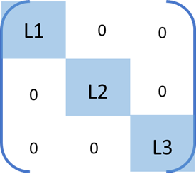
In this case, the three lowest eigenvalue-eigenvector pair of the Laplacian correspond to different clusters.
Algorithm
The way the Spectral Clustering algorithm works is:
- The first step is to build the Adjacency Matrix (A) from the given data points. For the data, we need to build the Similarity Graph which would be represented by the Adjacency Matrix. There are various methods to do so, such as Epsilon-neighbourhood Graph , using K-Nearest Neighbours , or building a Fully-Connected Graph .
- The next step is to compute the Degree Matrix (D) for the graph
- Then, the Graph Laplacian matrix is computed by doing L = D – A.
- The data needs to be projected to a low-dimensional space. Eigenvalues and their respective eigenvectors are calculated. Suppose the optimal number of clusters is c , then the first c eigenvalues and their corresponding eigenvectors are taken. These are then put into a matrix where the columns are the eigenvectors.
- After this, each node in the data is given a row of the Graph Laplacian Matrix.
- Then any clustering technique is applied to this reduced data.
Example
Let’s take a look at an example of Spectral Clustering in Python. The function SpectralClustering() is present in Python’s sklearn library.
Consider the following data:
from sklearn.datasets import make_circles
from sklearn.preprocessing import StandardScaler
create the datase
x, y = make_circles(n_samples=1000, factor=0.5, noise=0.06)
normalization of the values
x = StandardScaler().fit_transform(x)
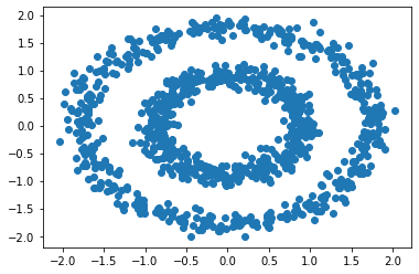
Here, we are creating data with points distributed in two concentric circles. The function used to create these data points is the make_circles() function. The parameters for this function for our data are – 1000 sample data points, factor=0.5, and noise=0.06 as defined in the code.
We can visualize these data points using matplotlib, as:
import matplotlib.pyplot as plt
plt.scatter(x[:,0], x[:,1])
plt.show()
The scatter plot is:
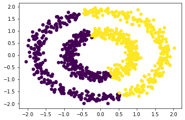
If we used the kMeans algorithm on this data, it would not segregate the clusters in the way we want. Let’s look at the clusters formed with kMeans, then we will compare it with Spectral Clustering.
from sklearn.cluster import KMeans
kmeans = KMeans(n_clusters=2).fit(x)
y2 = kmeans.predict(x)
plot
plt.scatter(x[:, 0], x[:, 1], c=y2)
plt.show()
The plot using kMeans is:
Now let’s apply the Spectral Clustering algorithm to the above data points. The python code to do so is:
from sklearn.cluster import SpectralClustering
model = SpectralClustering(n_clusters=2, affinity=’nearest_neighbors’).fit(x)
Here, for the algorithm, we have specified the number of clusters = 2.
Let’s visualize how the points are classified in the clusters:
y2 = model.fit_predict(x)
plt.scatter(x[:, 0], x[:, 1], c=y2)
plt.show()
The scatter plot with Spectral Clustering is:
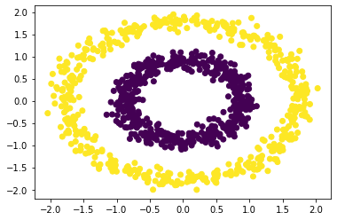
We can see that the algorithm has identified the clusters.
Summary
In this article, we focused on Spectral Clustering.