Python Implementation of Hierarchical Clustering

[vishrut-singhal]

Steps for implementation of AHC using Python:

The steps for implementation will be the same as the k-means clustering, except for some changes such as the method to find the number of clusters. Below are the steps:

1. Data Pre-processing
2. Finding the optimal number of clusters using the Dendrogram
3. Training the hierarchical clustering model
4. Visualizing the clusters

Data Pre-processing Steps:

In this step, we will import the libraries and datasets for our model.

• Importing the libraries

1. Importing the libraries

2. import numpy as nm
3. import matplotlib.pyplot as mtp
4. import pandas as pd

The above lines of code are used to import the libraries to perform specific tasks, such as numpy for the Mathematical operations, matplotlib for drawing the graphs or scatter plot, and pandas for importing the dataset.

• Importing the dataset

1. Importing the dataset

2. dataset = pd.read_csv(‘Mall_Customers_data.csv’)

As discussed above, we have imported the same dataset of Mall_Customers_data.csv, as we did in k-means clustering. Consider the below output:

• Extracting the matrix of features

Here we will extract only the matrix of features as we don’t have any further information about the dependent variable. Code is given below:

1. x = dataset.iloc[:, [3, 4]].values

Here we have extracted only 3 and 4 columns as we will use a 2D plot to see the clusters. So, we are considering the Annual income and spending score as the matrix of features.

Step-2: Finding the optimal number of clusters using the Dendrogram

Now we will find the optimal number of clusters using the Dendrogram for our model. For this, we are going to use scipy library as it provides a function that will directly return the dendrogram for our code. Consider the below lines of code:

1. #Finding the optimal number of clusters using the dendrogram
2. import scipy.cluster.hierarchy as shc
3. dendro = shc.dendrogram(shc.linkage(x, method=“ward”))
4. mtp.title(“Dendrogrma Plot”)
5. mtp.ylabel(“Euclidean Distances”)
6. mtp.xlabel(“Customers”)
7. mtp.show()

In the above lines of code, we have imported the hierarchy module of scipy library. This module provides us a method shc.denrogram(), which takes the linkage() as a parameter. The linkage function is used to define the distance between two clusters, so here we have passed the x(matrix of features), and method " ward ," the popular method of linkage in hierarchical clustering.

The remaining lines of code are to describe the labels for the dendrogram plot.

Output:

By executing the above lines of code, we will get the below output :

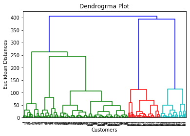
Using this Dendrogram, we will now determine the optimal number of clusters for our model. For this, we will find the maximum vertical distance that does not cut any horizontal bar. Consider the below diagram:

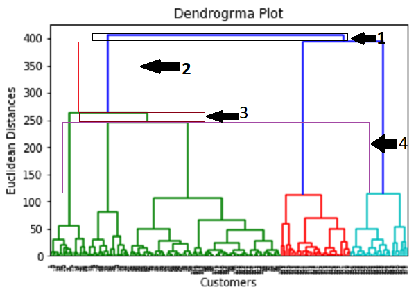
In the above diagram, we have shown the vertical distances that are not cutting their horizontal bars. As we can visualize, the 4th distance is looking the maximum, so according to this, the number of clusters will be 5 (the vertical lines in this range). We can also take the 2nd number as it approximately equals the 4th distance, but we will consider the 5 clusters because the same we calculated in the K-means algorithm.

So, the optimal number of clusters will be 5 , and we will train the model in the next step, using the same.

Step-3: Training the hierarchical clustering model

As we know the required optimal number of clusters, we can now train our model. The code is given below:

1. #training the hierarchical model on dataset
2. from sklearn.cluster import AgglomerativeClustering
3. hc= AgglomerativeClustering(n_clusters=5, affinity=‘euclidean’, linkage=‘ward’)
4. y_pred= hc.fit_predict(x)

In the above code, we have imported the AgglomerativeClustering class of cluster module of scikit learn library.

Then we have created the object of this class named as hc. The AgglomerativeClustering class takes the following parameters:

• n_clusters=5 : It defines the number of clusters, and we have taken here 5 because it is the optimal number of clusters.
• affinity=‘euclidean’ : It is a metric used to compute the linkage.
• linkage=‘ward’ : It defines the linkage criteria, here we have used the “ward” linkage. This method is the popular linkage method that we have already used for creating the Dendrogram. It reduces the variance in each cluster.

In the last line, we have created the dependent variable y_pred to fit or train the model. It does train not only the model but also returns the clusters to which each data point belongs.

After executing the above lines of code, if we go through the variable explorer option in our Sypder IDE, we can check the y_pred variable. We can compare the original dataset with the y_pred variable. Consider the below image:

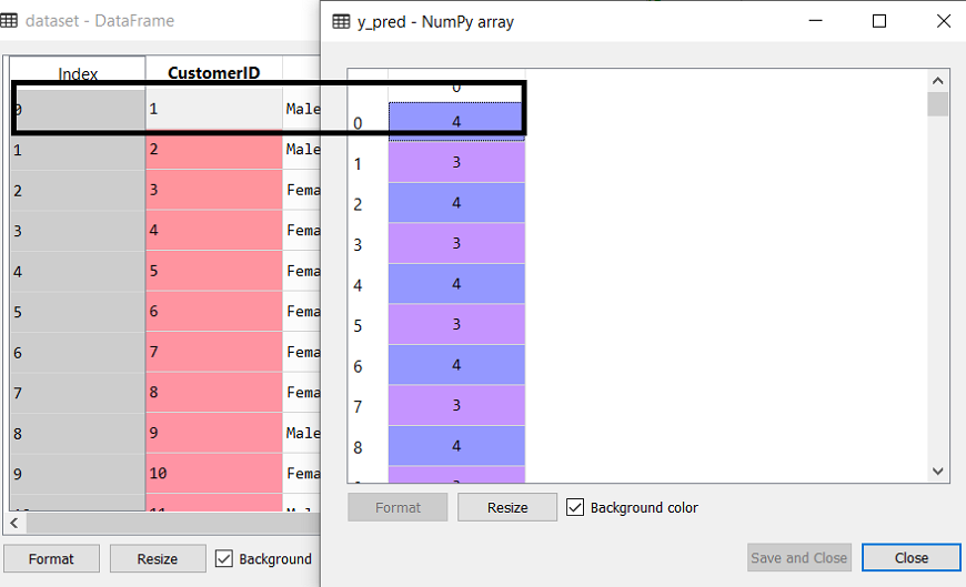
As we can see in the above image, the y_pred shows the clusters value, which means the customer id 1 belongs to the 5th cluster (as indexing starts from 0, so 4 means 5th cluster), the customer id 2 belongs to 4th cluster, and so on.

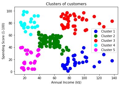
Step-4: Visualizing the clusters

As we have trained our model successfully, now we can visualize the clusters corresponding to the dataset.

Here we will use the same lines of code as we did in k-means clustering, except one change. Here we will not plot the centroid that we did in k-means, because here we have used dendrogram to determine the optimal number of clusters. The code is given below:

1. #visulaizing the clusters
2. mtp.scatter(x[y_pred == 0, 0], x[y_pred == 0, 1], s = 100, c = ‘blue’, label = ‘Cluster 1’)
3. mtp.scatter(x[y_pred == 1, 0], x[y_pred == 1, 1], s = 100, c = ‘green’, label = ‘Cluster 2’)
4. mtp.scatter(x[y_pred== 2, 0], x[y_pred == 2, 1], s = 100, c = ‘red’, label = ‘Cluster 3’)
5. mtp.scatter(x[y_pred == 3, 0], x[y_pred == 3, 1], s = 100, c = ‘cyan’, label = ‘Cluster 4’)
6. mtp.scatter(x[y_pred == 4, 0], x[y_pred == 4, 1], s = 100, c = ‘magenta’, label = ‘Cluster 5’)
7. mtp.title(‘Clusters of customers’)
8. mtp.xlabel(‘Annual Income (k$)’)
9. mtp.ylabel(‘Spending Score (1-100)’)
10. mtp.legend()
11. mtp.show()

Output: By executing the above lines of code, we will get the below output: