Key Concepts in Calculus: Rate of Change

[swapneel-panda-419bc751 (Swapneel Panda)]

The rate of change defines the relationship of one changing variable with respect to another.

Consider a moving object that is displacing twice as much in the vertical direction, denoted by y, as it is in the horizontal direction, denoted by x. In mathematical terms, this may be expressed as:

𝛿y = 2𝛿x

The Greek letter delta, 𝛿, is often used to denote difference or change. Hence, the equation above defines the relationship between the change in the x-position with respect to the change in the y-position of the moving object.

This change in the x and y-directions can be graphed by a straight line on an x–y coordinate system.

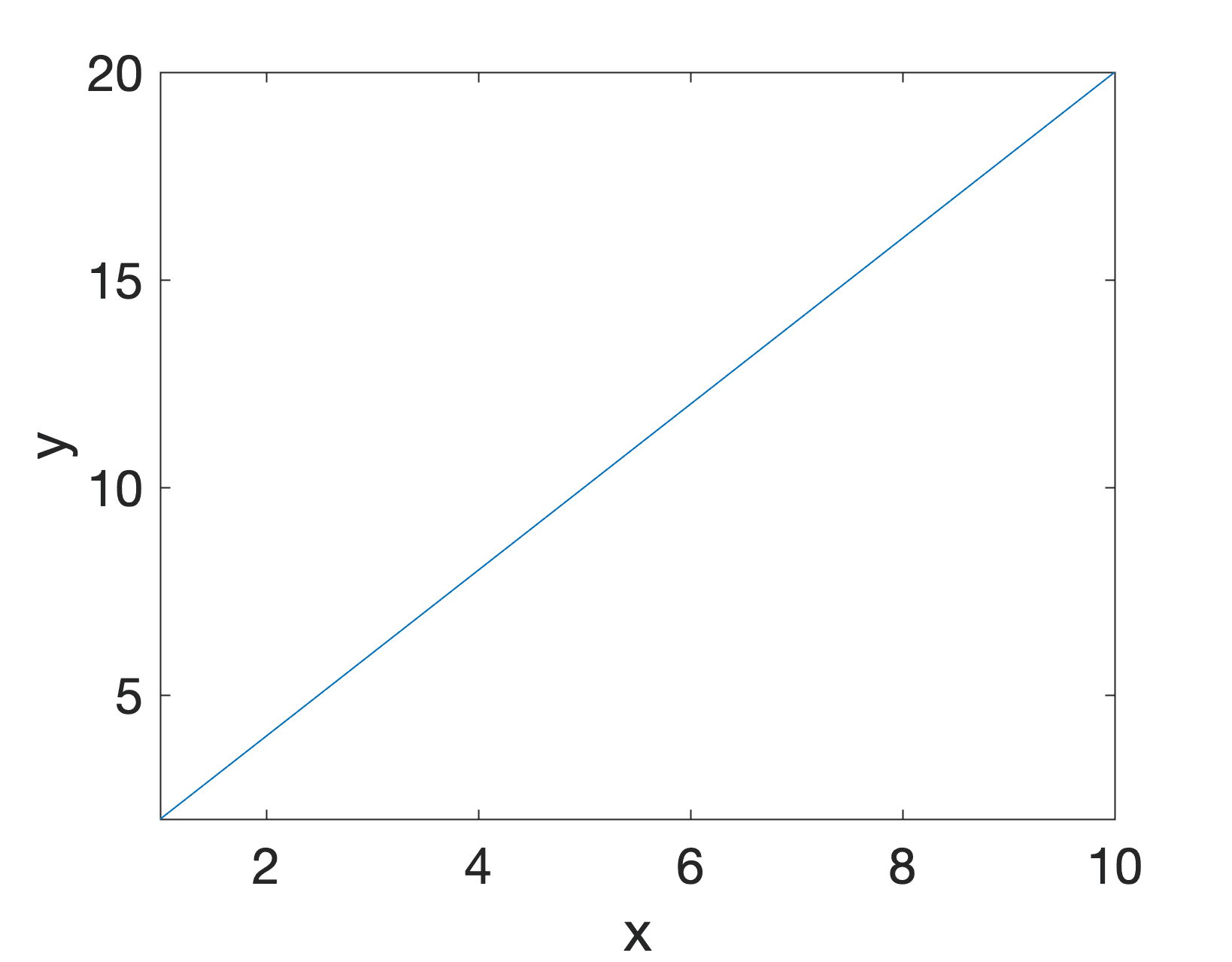
Line Plot of a Linear Function

In this graphical representation of the object’s movement, the rate of change is represented by the slope of the line, or its gradient. Since the line can be seen to rise 2 units for each single unit that it runs to the right, then its rate of change, or its slope, is equal to 2.

Rates and slopes have a simple connection. The previous rate examples can be graphed on an x-y coordinate system, where each rate appears as a slope.

Page 38, Calculus Essentials for Dummies, 2019.

Tying everything together, we see that:

rate of change = 𝛿y / 𝛿x = rise / run = slope

If we had to consider two particular points, P 1 = (2, 4) and P 2 = (8, 16), on this straight line, we may confirm the slope to be equal to:

slope = 𝛿y / 𝛿x = (y 2 – y 1) / (x 2 – x 1) = (16 – 4) / (8 – 2) = 2

For this particular example, the rate of change, represented by the slope, is positive since the direction of the line is increasing rightwards. However, the rate of change can also be negative if the direction of the line decreases, which means that the value of y would be decreasing as the value of x increases. Furthermore, when the value of y remains constant as x increases, we would say that we have zero rate of change. If, otherwise, the value of x remains constant as y increases, we would consider the range of change to be infinite, because the slope of a vertical line is considered undefined.

So far, we have considered the simplest example of having a straight line, and hence a linear function, with an unchanging slope. Nonetheless, not all functions are this simple, and if they were, there would be no need for calculus.

Calculus is the mathematics of change, so now is a good time to move on to parabolas, curves with changing slopes.

Page 39, Calculus Essentials for Dummies, 2019.

Let us consider a simple non-linear function, a parabola:

y = (1 / 4) x 2

In contrast to the constant slope that characterises a straight line, we may notice how this parabola becomes steeper and steeper as we move rightwards.

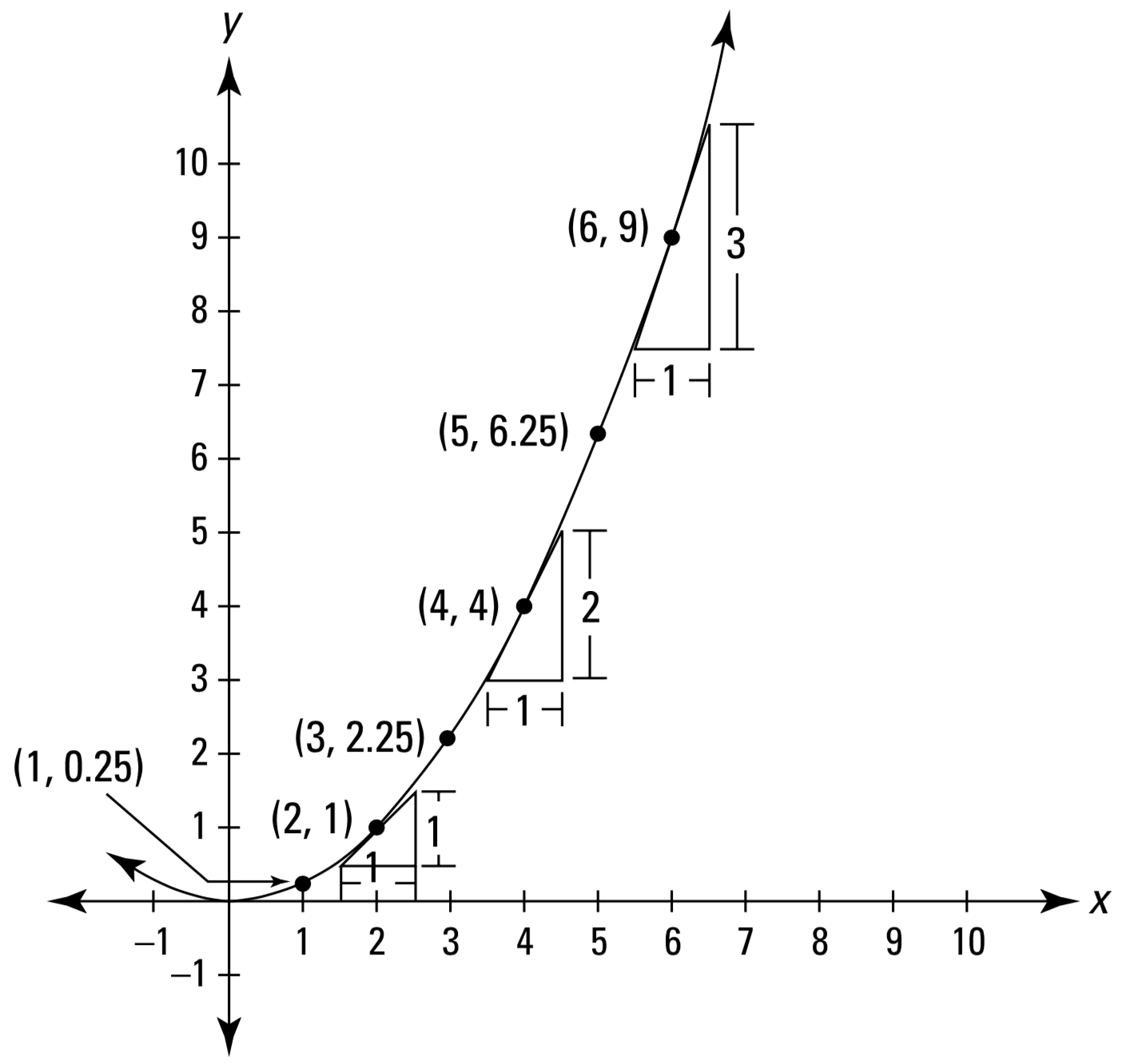
Line Plot of a Parabola
Taken from Calculus Essentials For Dummies

Recall that the method of calculus allows us to analyse a curved shape by cutting it into many infinitesimal straight pieces arranged alongside one another. If we had to consider one of such pieces at some particular point, P, on the curved shape of the parabola, we see that we find ourselves calculating again the rate of change as the slope of a straight line. It is important to keep in mind that the rate of change on a parabola depends on the particular point, P, that we happened to consider in the first place.

For example, if we had to consider the straight line that passes through point, P = (2, 1), we find that the rate of change at this point on the parabola is:

rate of change = 𝛿y / 𝛿x = 1 / 1 = 1

If we had to consider a different point on the same parabola, at P = (6, 9), we find that the rate of change at this point is equal to:

rate of change = 𝛿y / 𝛿x = 3 / 1 = 3

The straight line that touches the curve as some particular point, P, is known as the tangent line, whereas the process of calculating the rate of change of a function is also known as finding its derivative.

A derivative is simply a measure of how much one thing changes compared to another — and that’s a rate.

Page 37, Calculus Essentials for Dummies, 2019.

While we have considered a simple parabola for this example, we may similarly use calculus to analyse more complicated non-linear functions. The concept of computing the instantaneous rate of change at different tangential points on the curve remains the same.

We meet one such example when we come to train a neural network using the gradient descent algorithm. As the optimization algorithm, gradient descent iteratively descends an error function towards its global minimum, each time updating the neural network weights to model better the training data. The error function is, typically, non-linear and can contain many local minima and saddle points. In order to find its way downhill, the gradient descent algorithm computes the instantaneous slope at different points on the error function, until it reaches a point at which the error is lowest and the rate of change is zero.