How to Freeze and Unfreeze Cells in Excel?

[vishrut-singhal]

Whenever you are working with large datasets in Excel, it can be difficult to compare your workbook information. You may often want to lock certain rows or columns so that you can view their contents while scrolling to another area of the worksheet.

Excel includes several tools that make it easier to view content from different parts of your workbook simultaneously, such as the ability to freeze panes and split your worksheet and a few other features of Excel.

Freezing rows or columns ensures that certain cells remain visible as you scroll through the data. If you want to easily edit two parts of the spreadsheet at once, splitting your panes will make the task much easier.

Freezing rows in [Excel] is a few clicks thing. You click on the View tab then Freeze Panes and choose one of the following options, depending on how many rows you want to lock:

• Freeze Top Row is used to lock the first row.
• Freeze Panes are used to lock several rows.

How to Freeze Top Row

Follow the following steps to lock the top row in Excel:

Step 1: Create a dataset on an excel worksheet as below.

Step 2: Go to the View tab and click Freeze Panes .

Step 3: Then select the Freeze Top Row from the dropdown list.

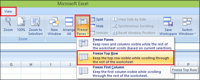
This will lock the very first row in your worksheet so that it remains visible when you navigate through the rest of your worksheet.

Step 4: Excel automatically adds a dark grey horizontal line to indicate that the top row is frozen.

Unfreeze Panes

To unlock or unfreeze the rows, execute the following steps.

Step 1: Click on the View tab in the Window group.

Step 2: And again click Freeze Panes .

Step 3: Then click on the Unfreeze Panes in the dropdown list.

After click on the Unfreeze Pane, it unlocks the first row and the worksheet change back to an old worksheet without any gray line.

How to Freeze Multiple Rows

In case you want to lock several rows, follow the following steps:

Step 1: Select the row or cell that you want to freeze.

Step 2: Click on the View tab and go on Freeze Panes .

Step 3: And again, click on the Freeze Panes in the dropdown list.

For example, to freeze the top three rows in Excel, we select cell A4 or the entire row.

Step 4: Now click Freeze Panes , and it gives the following worksheet with a gray line after the three rows.

NOTE: Microsoft Excel allows freezing only rows at the top of the spreadsheet. It is not possible to lock rows in the middle of the sheet. Make sure that all the rows to be locked are visible at the moment of freezing.

How to Freeze the First Column

To freeze the first column, execute the following steps.

Step 1: Click on the View tab in the Window group.

Step 2: Go to Freeze Panes .

Step 3: And click on the Freeze First Column in the dropdown list.

Step 4: Scroll to the right of the worksheet.

Step 5: Excel automatically adds a dark grey vertical line to indicate that the first column is frozen.

How to Freeze Multiple Columns

In case you want to freeze more than one column, this is what you need to do:

Step 1: Select the column or the first cell in the column to the right of the last column you want to lock.

For example, to freeze the first two columns, select the whole column C or cell C1.

Step 2: Click on the View tab.

Step 3: Go to the Freeze Panes .

Step 4: And click on the Freeze Panes in the dropdown list.

Step 5: It will lock the first two columns in place, as indicated by the thicker and darker border, enabling you to view the cells in frozen columns as you move across the worksheet.

NOTE: You can only freeze columns on the left side of the sheet. You cannot freeze Columns in the middle of the worksheet. All the columns to be locked should be visible . Any columns that are out of view will be hidden after freezing.

How to Freeze Cells

Besides locking columns and rows separately, Microsoft Excel lets you freeze both rows and columns simultaneously. You need to follow the following steps to freeze the cells or rows and columns both:

Step 1: Select a cell below the last row and the right of the last column you need to freeze.

For example, if you want to freeze the top row and first column in a single step, select cell B2.

Step 2: Click on the View tab.

Step 3: Go to the Freeze Panes .

Step 4: And click on the Freeze Panes in the dropdown list.

Step 5: The header row and leftmost column of your table will always be viewable as you scroll down and to the right.

Similarly, you can freeze as many rows and columns as you want as long as you start with the top row and leftmost column.

For example, if you want to lock the first two rows and the first two columns, then you need to select cell C3 and so on.

Freeze Panes not working

If the Freeze Panes button is disabled or grayed out in your worksheet, most probable it is because of the following reasons:

• For example, in cell editing mode, you enter a formula or editing data in a cell. To exit cell editing mode, press the Enter or Esc
• Your worksheet is protected. First, you need to remove the workbook protection and then freeze rows or columns.

Magic Freeze Button

Add the magic Freeze button to the Quick Access Toolbar to freeze the top row, the first column, rows, columns or cells with a single click.

Step 1: Click the down arrow and click on the More Commands in the dropdown list.

Step 2: Under Choose commands from, select Commands Not in the Ribbon.

Step 3: Select Freeze Sheet Panes and click on the Add button.

Step 4: Now click on the Ok button.

Step 5: Freeze Sheet Panes icon appears on the top and right side of the down arrow.

For example, if you want to freeze the top four rows and first column, select B5 cell and click the magic Freeze button.

Excel automatically adds a dark grey horizontal and vertical line to indicate that the rows and columns are frozen.

Other Ways to Freeze Columns and Rows

Apart from freezing panes, Microsoft Excel provides a few more ways to freeze certain sheet areas.

1. Split panes

Another way to freeze cells in Excel is to split a worksheet area into several parts. The difference is as follows:

Freezing panes allows you to keep certain rows or/and columns visible when scrolling across the worksheet.

Splitting panes divides the Excel window into two or four areas that can be scrolled separately. When you scroll within one area, the cells in the other area(s) remain fixed.

To split Excel’s worksheet, follow the following steps:

Step 1: Select a cell where you want the split in the worksheet.

Step 2: Click the View tab in the window group.

Step 3: And click on the Split button.

Step 4: It horizontally split the worksheet into two sections, as shown below.

If you want to undo a split, again click on the Split button.

2. Use Tables to Lock-Top Row

If you want to lock the header row and always stay fixed at the top while you scroll down, convert a range to a fully-functional Excel table.

Step 1: In excel, the fastest way to create a table is by pressing the Ctrl + T shortcut key.

Step 2: Then, a Create Table dialog box appears. Click the Ok button.

Step 3: This lock or freeze the header row of the table while you scroll down.

3. Print header rows on every page

If you want to repeat the top row or rows on every printed page, then, in this case, you need to follow the following basic steps:

Step 1: First, click on the Page Layout tab.

Step 2: And click on the Print Titles button.

Step 3: Then, a Page Setup dialog box appears.

Step 4: Select rows to repeat and enter them in the Rows to repeat at the top box.

This repeats the top row on every printed page of the excel worksheet.