nstallation
For analysis, we need to install the GreyKite library. Check the below command to install the library. Type the below command in the command line prompt. For more information, check the below code.
%matplotlib inline !pip install -qqq greykite
Import Libraries
In this section, we are going to import all the required libraries that are useful for further analysis. We will be using Pandas, collections, plotly, matplotlib, and Greykite. For more information, check the below code.
from collections import defaultdict import warnings import pandas as pd warnings.filterwarnings(“ignore”) import pandas as pd import plotly from greykite.framework.templates.autogen.forecast_config import ForecastConfig from greykite.framework.templates.autogen.forecast_config import MetadataParam from greykite.framework.templates.forecaster import Forecaster from greykite.framework.templates.model_templates import ModelTemplateEnum from greykite.framework.utils.result_summary import summarize_grid_search_results
Read Dataset
In this section, we are going to read data. We are using Pandas read_csv() function. I am changing the data type of the DATE parameter using astype() function. After this, rename the column DATE as ts and Value as y. We are using the head() function and passing the parameter 100 to show the first 100 rows of the dataset. Check the below code for more information.
df = pd.read_csv(‘electric-production/Electric_Production.csv’) df[‘DATE’] = df[‘DATE’].astype(‘datetime64[ns]’) df.rename(columns = {‘DATE’: ‘ts’, ‘Value’: ‘y’}, inplace = True) df = df.head(100) df

Create a Forecast
The forecast can be created with just a few lines of code. First, specify the dataset information. We are setting the time_col parameter as ts and the value_col parameter as y . In freq, we are setting value as MS for Monthly at the start date. After this create a forecaster using the Forecaster class from the GreyKite package. The output of run_forecast_config() would be a dictionary which is having future predicted values, original time series, and historical forecast performance. Check the below code for complete information.
Specifies dataset information metadata = MetadataParam( time_col=“ts”, # name of the time column value_col=“y”, # name of the value column freq=“MS” #“MS” for Montly at start date, “H” for hourly, “D” for daily, “W” for weekly, etc. ) forecaster = Forecaster() result = forecaster.run_forecast_config( df=df, config=ForecastConfig( model_template=ModelTemplateEnum.SILVERKITE.name, forecast_horizon=100, # forecasts 100 steps ahead coverage=0.95, # 95% prediction intervals metadata_param=metadata ) )

ts = result.timeseries fig = ts.plot() plotly.io.show(fig)

Cross-Validation
As a matter of course, run_forecast_config gives chronicled assessment, so you can perceive how the conjecture performs on past information. This is put away in grid_search (cross-approval parts) and backtest (holdout test set).
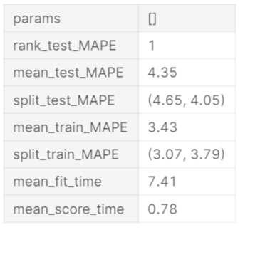
How about we check the cross-validation results. Naturally, all measurements in Element-wise Evaluation Metric Enum are registered on every CV train/test split. The setup of CV assessment measurements can be found at Evaluation Metric. Underneath, we show the Mean Absolute Percentage Error (MAPE) across parts
grid_search = result.grid_search cv_results = summarize_grid_search_results( grid_search=grid_search, decimals=2, # The below saves space in the printed output. Remove to show all available metrics and columns. cv_report_metrics=None, column_order=[“rank”, “mean_test”, “split_test”, “mean_train”, “split_train”, “mean_fit_time”, “mean_score_time”, “params”]) # Transposes to save space in the printed output cv_results[“params”] = cv_results[“params”].astype(str) cv_results.set_index(“params”, drop=True, inplace=True) cv_results.transpose()
Backtest
Let’s plot the historical forecast on the holdout test set. Check the below code for more information.
backtest = result.backtest fig = backtest.plot() plotly.io.show(fig)

Check the historical evaluation metrics(on the historical test/train set) using the below code
backtest_eval = defaultdict(list) for metric, value in backtest.train_evaluation.items(): backtest_eval[metric].append(value) backtest_eval[metric].append(backtest.test_evaluation[metric]) metrics = pd.DataFrame(backtest_eval, index=[“train”, “test”]).T metrics

Forecast
In this section, we are going to plot the forecasted values. The forecast attribute having a forecasted value. Let’s plot the forecasted values using the below code. For more information, check the below code.
forecast = result.forecast fig = forecast.plot() plotly.io.show(fig)

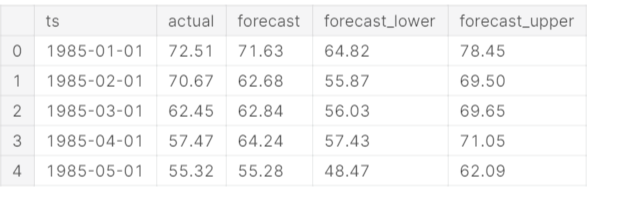
You can also check the forecasted values using the head() function. All the forecasted values are there in df. For more information, check the below code.
forecast.df.head().round(2)
Model Diagnostics
In this section, we are going to see model diagnostics. There are one more plot function plot_components() , this plot shows how your dataset’s trend, event/holiday, seasonality patterns are handled in the model. For more information, check the below code.
fig = forecast.plot_components() plotly.io.show(fig) # fig.show() if you are using “PROPHET” template

The model summary allows inspection of individual model terms. Check parameter estimates and their significance for insights on how the model works and what can be further improved.
summary = result.model[-1].summary() # -1 retrieves the estimator from the pipeline print(summary)
