FV() function in Excel

[vishrut-singhal]

FV() is an in-built Excel function used for financial calculation. Here, FV() refers to the Future Value. This function helps to calculate the compound interest and return future value.

Before detailing of FV() function, you need to know little about compound interest and its basic terms. As it is used for calculating the compound interest and future value for further year interest calculation.

In this chapter, we are going to describe the FV() function in detail with its syntax, parameters, and examples.

What is compound interest?

Compound interest is an amount that is calculated over the principal amount in the first year and then with interest over interest. The user must know the compound interest, its basic terms, and usage. If the user has good knowledge of compound interest and its formulas, one can more easily and faster learn and use Excel’s FV() function.

Understand compound interest in the simplest language or term, i.e., “Interest over interest”.

Although we have provided a detailed description about compound interest and its manual calculation in the previous chapter. But it can also be calculated through the Excel in-built method. Excel offers FV() function, which is an in-built Excel function used to calculate compound interest.

FV() function

FV() refers to the Future Value. It is a built-in function of Excel that is used to calculate the compound interest on some value. Similar to manual compound interest methods, it also calculates the future value on an investment. This function is a bit tricky to understand.

Compound interest is the base of the FV() function. It can be calculated periodically, like - monthly, quarterly, semi-year, or annually. Provide the data accordingly.

Syntax

Compound interest takes five arguments, in which the last two are optional. Firstly, see the syntax then we will talk about its parameters.

=FV(rate, nper, pmt, [pv], [type])

Each parameter belongs to a specific value of compound interest, such as -

Parameter	Description
rate (required)	The rate parameter contains the interest rate to be applied to an amount for each period.
nper (required)	It contains the number of compounding periods per year. The compounding period means how many times interest given to the user in a year. It can be monthly, quarterly, or annually.
pmt (required)	The pmt is an additional amount per period. It is represented as a negative number. It means that the value must be a negative number. If there is no value in pmt, then put 0 as its value.
pv (optional)	Pv refers to the principal investment, which is an optional parameter value. Like the pmt, if there is no value in pv, put 0 as its value.
type (optional)	This parameter is passed when payments are due. It is also an optional argument whose default value is 0. Here, 0 stands for end of the period and 1 for beginning of the period.

Return value

The FV() function of Excel returns the future value on investment. On which the calculation of compound interest depends for further years.

Example 1: Compound interest with no compounding period

Let’s take an example and understand how FV() function works with its parameters. Before we will describe a simple scenario:

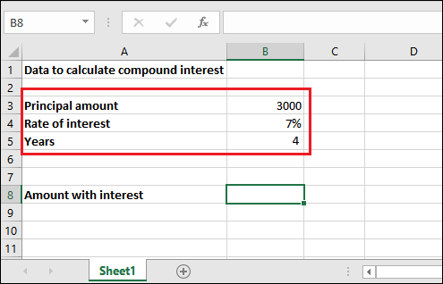
Question

We have deposited 3000 rupees for 4 years at 7% of annual interest rate compounded yearly. It means the compounding period value will be 1 by default, or you can suppose it as no additional compounding period.

Solution

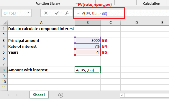
For this problem, we will put the given values inside the FV() formula directly without any extra calculation and get the compound interest calculated for 4 years.

Hence, the FV() formula goes like -

=FV(B4, B5, ,-B3)

Select the cell reference for the value accordingly. Do not copy ours.

Or

=FV(7%, 4, ,-3000)

• pmt value is empty here because no additional payments are defined in the question.

Steps to calculate compound interest

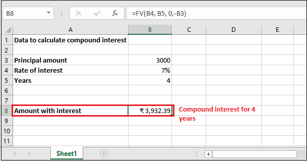
Step 1: Select the cell to keep the calculated result and write the created FV() formula in the formula bar.

=FV(B4, B5, ,-B3)

Step 2: Get the Balance returned with interest by pressing the Enter key. See that it returned interest added with principal amount is 3932.39 for all four years.

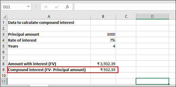
Step 3: You can extract the interest only from the returned amount by subtracting the initial investment (principal amount) from it. See the result - 932.39 compound interest over 3000 rupees.

Example 2: Compound interest with compounding period

Question

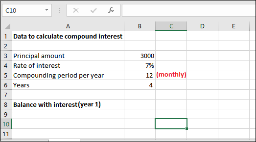
We have the same problem as the above example. We have deposited 3000 rupees for 4 years at 7% of annual interest rate compounded monthly. It means - this time compounding period is monthly, whose value will be 12. There is no additional payment.

See the dataset below:

Solution

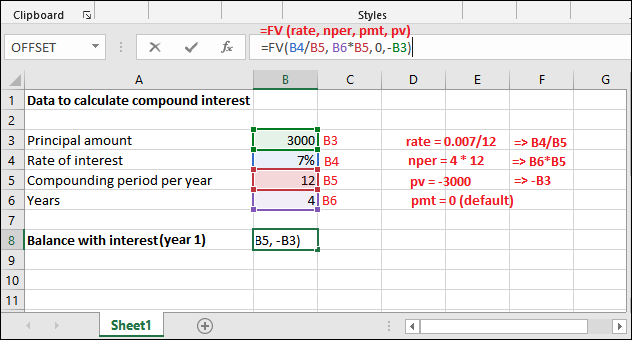
This time, FV() function requires some extra calculation than passing the parameter values directly. Hence, the FV() formula goes like -

=FV(B4/B5, B6*B5, 0, -B3)

You can also provide these values directly into the formula instead of cell reference.

=FV(0.007/12, 4*12, 0, -3000)

"Remember, this formula will calculate the compound interest for one year with monthly compounding period. You have to calculate compound interest for each year with new future value received through previous year calculation."

Now, see the detailed explanation;

1. Here, the rate parameter will have 0.007/12. Since, the interest rate is 7% per year compounded monthly (12 months in a year), as you mentioned above.
2. For nper, the value will be 4 * 12, i.e., 4 years* 12 months, because the compounding period is monthly.
3. The pmt parameter will remain empty as there is no additional payments included.
4. Pv value will be -3000 as the pv is represented as a negative number.

Steps to calculate compound interest

Step 1: Select the cell to keep the calculated result and write the created FV() formula in the formula bar.

=FV(B4/B5, B6*B5, 0, -B3)

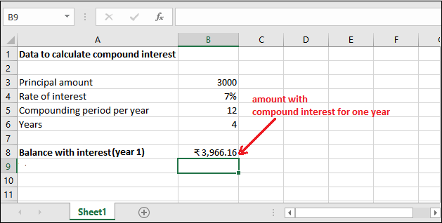
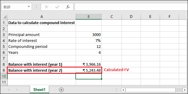
Step 2: Get the Balance returned with interest by pressing the Enter key. See that the returned future value amount is 3966.16 for 1-year with monthly compounding period.

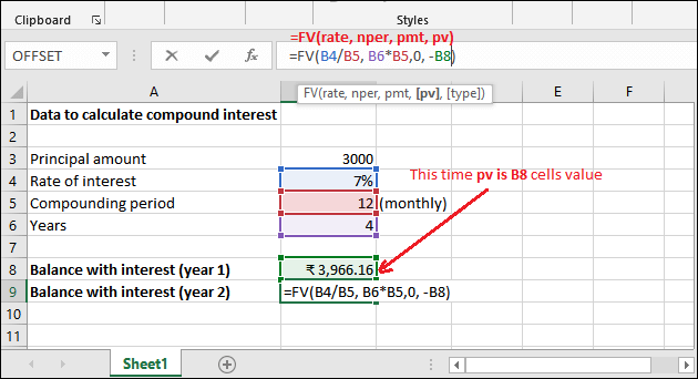
Year 2

Step 3: Now, we will calculate the interest for year 2 with the new Future Value returned in the previous step.

=FV(B4/B5, B6*B5,0, -B8)

Step 4: Get the calculated compound interest (future value) for year 2, i.e., 5243.48.

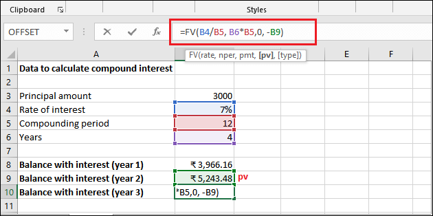
Year 3

Step 5: Using the following formula, we will calculate the interest for year 3 with the new Future Value returned in the previous step.

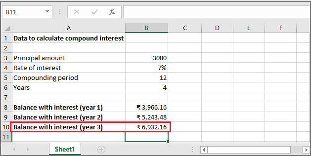
=FV(B4/B5, B6*B5,0, -B9)

Step 6: Get the calculated compound interest (future value) for year 3, which is 6932.16

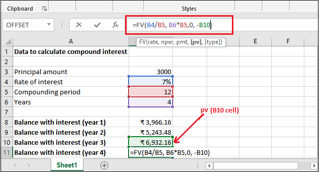
Year 4

Step 7: Using the following formula, we will calculate the interest for year 4 with the new Future Value returned in the previous step.

=FV(B4/B5, B6*B5,0, -B10)

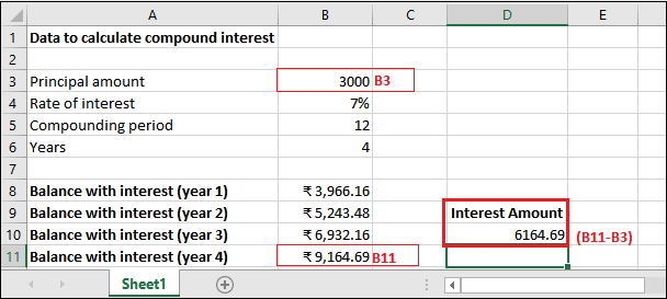
Step 8: Get the calculated compound interest (future value) for year 4, which is 9164.69.

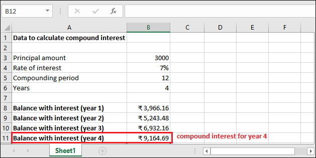
You can extract only the compound interest from the final amount returned after four years with a monthly compounding period. See the result that only interest is 6164.69.

Similarly, you can count the compound interest for another dataset.

Another FV() formula

Look at one more example for FV() function using a simple and easily understandable FV() formula. If the previously used formula is difficult to understand. Remember, it works completely same.

=FV(R/N, Y*N,-P)

Here,

• R is the annual interest rate.
• N is the number of compounding periods per year. For example , your compounding period is annual, N will be 1. Similarly, if the compounding period is quarterly, N will be 4 and if the compounding period is monthly, N will be 12.
• Y is number of years to calculate interest.
• P is the initial investment means the principal amount, which is always used as a negative number in this function. This principal amount value changes every year, which is future value returned by the FV().

Note: Present value (principal amount) is always be negative for this function because there is a negative relationship between present value and future value.

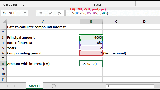
Example 3

We have deposited 4000 rupees for 2 years at 8% of annual interest rate with a semi-annual compounding period. Remember that - there is no additional payment.

Steps to calculate compound interest

Step 1: Select the cell to keep the calculated result and write the created FV() formula in the formula bar.

=FV(B4/B6, B5*B6, 0,-B3)

Step 2: Get the Balance returned with interest by pressing the Enter key. See that it returned interest with principal amount is 4679.43 for 1st year.

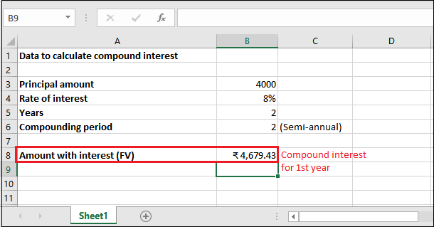
Step 3: Only interest amount for the first year is 679.43. Since, it can get by subtracting principal amount from future value, i.e., Principal amount - Future Value.

Similarly, you can calculate for the other years by using a new future value.