Central Limit Theorem Concept

[ashish-singh-2f6974d6 (Ashish Singh)]

The central limit theorem states that if you have a population with mean μ and standard deviation σ and take sufficiently large random samples from the population with replacement, then the distribution of the sample means will be approximately normally distributed. This will hold true regardless of whether the source population is normal or skewed, provided the sample size is sufficiently large (usually n > 30). If the population is normal, then the theorem holds true even for samples smaller than 30. In fact, this also holds true even if the population is binomial, provided that min(np, n(1-p))> 5, where n is the sample size and p is the probability of success in the population. This means that we can use the normal probability model to quantify uncertainty when making inferences about a population mean based on the sample mean.

For the random samples we take from the population, we can compute the mean of the sample means:

and the standard deviation of the sample means:

Before illustrating the use of the Central Limit Theorem (CLT) we will first illustrate the result. In order for the result of the CLT to hold, the sample must be sufficiently large (n > 30). Again, there are two exceptions to this. If the population is normal, then the result holds for samples of any size (i…e, the sampling distribution of the sample means will be approximately normal even for samples of size less than 30).

Central Limit Theorem with a Normal Population

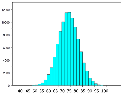
The figure below illustrates a normally distributed characteristic, X, in a population in which the population mean is 75 with a standard deviation of 8.

If we take simple random samples (with replacement) of size n=10 from the population and compute the mean for each of the samples, the distribution of sample means should be approximately normal according to the Central Limit Theorem. Note that the sample size (n=10) is less than 30, but the source population is normally distributed, so this is not a problem. The distribution of the sample means is illustrated below. Note that the horizontal axis is different from the previous illustration, and that the range is narrower.

The mean of the sample means is 75 and the standard deviation of the sample means is 2.5, with the standard deviation of the sample means computed as follows:

If we were to take samples of n=5 instead of n=10, we would get a similar distribution, but the variation among the sample means would be larger. In fact, when we did this we got a sample mean = 75 and a sample standard deviation = 3.6.