A neural network model, whether shallow or deep, implements a function that maps a set of inputs to expected outputs.
The function implemented by the neural network is learned through a training process, which iteratively searches for a set of weights that best enable the neural network to model the variations in the training data.
A very simple type of function is a linear mapping from a single input to a single output.
Page 187, Deep Learning, 2019.
Such a linear function can be represented by the equation of a line having a slope, m, and a y-intercept, c:
y = mx + c
Varying each of parameters, m and c, produces different linear models that define different input-output mappings.

Line Plot of Different Line Models Produced by Varying the Slope and Intercept
Taken from Deep Learning
The process of learning the mapping function, therefore, involves the approximation of these model parameters, or weights, that result in the minimum error between the predicted and target outputs. This error is calculated by means of a loss function, cost function, or error function, as often used interchangeably, and the process of minimizing the loss is referred to as function optimization.
We can apply differential calculus to the process of function optimization.
In order to understand better how differential calculus can be applied to function optimization, let us return to our specific example of having a linear mapping function.
Say that we have some dataset of single input features, x, and their corresponding target outputs, y. In order to measure the error on the dataset, we shall be taking the sum of squared errors (SSE), computed between the predicted and target outputs, as our loss function.
Carrying out a parameter sweep across different values for the model weights, w0 = m and w1 = c, generates individual error profiles that are convex in shape.

Line Plots of Error (SSE) Profiles Generated When Sweeping Across a Range of Values for the Slope and Intercept
Taken from Deep Learning
Combining the individual error profiles generates a three-dimensional error surface that is also convex in shape. This error surface is contained within a weight space, which is defined by the swept ranges of values for the model weights, w0 and w1.
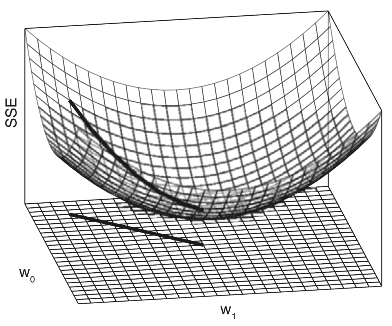
Three-Dimensional Plot of the Error (SSE) Surface Generated When Both Slope and Intercept are Varied
Taken from Deep Learning
Moving across this weight space is equivalent to moving between different linear models. Our objective is to identify the model that best fits the data among all possible alternatives. The best model is characterised by the lowest error on the dataset, which corresponds with the lowest point on the error surface.
A convex or bowl-shaped error surface is incredibly useful for learning a linear function to model a dataset because it means that the learning process can be framed as a search for the lowest point on the error surface. The standard algorithm used to find this lowest point is known as gradient descent.
Page 194, Deep Learning, 2019.
The gradient descent algorithm, as the optimization algorithm, will seek to reach the lowest point on the error surface by following its gradient downhill. This descent is based upon the computation of the gradient, or slope, of the error surface.
This is where differential calculus comes into the picture.
Calculus, and in particular differentiation, is the field of mathematics that deals with rates of change.
Page 198, Deep Learning, 2019.
More formally, let us denote the function that we would like to optimize by:
error = f(weights)
By computing the rate of change, or the slope, of the error with respect to the weights, the gradient descent algorithm can decide on how to change the weights in order to keep reducing the error.