What is Backward Elimination?
Backward elimination is a feature selection technique while building a machine learning model. It is used to remove those features that do not have a significant effect on the dependent variable or prediction of output. There are various ways to build a model in Machine Learning, which are:
- All-in
- Backward Elimination
- Forward Selection
- Bidirectional Elimination
- Score Comparison
Above are the possible methods for building the model in Machine learning, but we will only use here the Backward Elimination process as it is the fastest method.
Steps of Backward Elimination
Below are some main steps which are used to apply backward elimination process:
Pause
Unmute
Loaded: 19.95%
Fullscreen
Step-1: Firstly, We need to select a significance level to stay in the model. (SL=0.05)
Step-2: Fit the complete model with all possible predictors/independent variables.
Step-3: Choose the predictor which has the highest P-value, such that.
- If P-value >SL, go to step 4.
- Else Finish, and Our model is ready.
Step-4: Remove that predictor.
Step-5: Rebuild and fit the model with the remaining variables.
Need for Backward Elimination: An optimal Multiple Linear Regression model:
In the previous chapter, we discussed and successfully created our Multiple Linear Regression model, where we took 4 independent variables (R&D spend, Administration spend, Marketing spend, and state (dummy variables)) and one dependent variable (Profit) . But that model is not optimal, as we have included all the independent variables and do not know which independent model is most affecting and which one is the least affecting for the prediction.
Unnecessary features increase the complexity of the model. Hence it is good to have only the most significant features and keep our model simple to get the better result.
So, in order to optimize the performance of the model, we will use the Backward Elimination method. This process is used to optimize the performance of the MLR model as it will only include the most affecting feature and remove the least affecting feature. Let’s start to apply it to our MLR model.
Steps for Backward Elimination method:
We will use the same model which we build in the previous chapter of MLR. Below is the complete code for it:
-
importing libraries
- import numpy as nm
- import matplotlib.pyplot as mtp
- import pandas as pd
- #importing datasets
- data_set= pd.read_csv(‘50_CompList.csv’)
- #Extracting Independent and dependent Variable
- x= data_set.iloc[:, :-1].values
- y= data_set.iloc[:, 4].values
- #Catgorical data
- from sklearn.preprocessing import LabelEncoder, OneHotEncoder
- labelencoder_x= LabelEncoder()
- x[:, 3]= labelencoder_x.fit_transform(x[:,3])
- onehotencoder= OneHotEncoder(categorical_features= [3])
- x= onehotencoder.fit_transform(x).toarray()
- #Avoiding the dummy variable trap:
- x = x[:, 1:]
-
Splitting the dataset into training and test set.
- from sklearn.model_selection import train_test_split
- x_train, x_test, y_train, y_test= train_test_split(x, y, test_size= 0.2, random_state=0)
- #Fitting the MLR model to the training set:
- from sklearn.linear_model import LinearRegression
- regressor= LinearRegression()
- regressor.fit(x_train, y_train)
- #Predicting the Test set result;
- y_pred= regressor.predict(x_test)
- #Checking the score
- print('Train Score: ', regressor.score(x_train, y_train))
- print('Test Score: ', regressor.score(x_test, y_test))
From the above code, we got training and test set result as:
Train Score: 0.9501847627493607 Test Score: 0.9347068473282446
The difference between both scores is 0.0154.
Note: On the basis of this score, we will estimate the effect of features on our model after using the Backward elimination process.
Step: 1- Preparation of Backward Elimination:
- Importing the library: Firstly, we need to import the statsmodels.formula.api library, which is used for the estimation of various statistical models such as OLS(Ordinary Least Square). Below is the code for it:
- import statsmodels.api as smf
-
Adding a column in matrix of features: As we can check in our MLR equation (a), there is one constant term b0, but this term is not present in our matrix of features, so we need to add it manually. We will add a column having values x0 = 1 associated with the constant term b0.
To add this, we will use append function of Numpy library (nm which we have already imported into our code), and will assign a value of 1. Below is the code for it.
- x = nm.append(arr = nm.ones((50,1)).astype(int), values=x, axis=1)
Here we have used axis =1, as we wanted to add a column. For adding a row, we can use axis =0.
Output: By executing the above line of code, a new column will be added into our matrix of features, which will have all values equal to 1. We can check it by clicking on the x dataset under the variable explorer option.
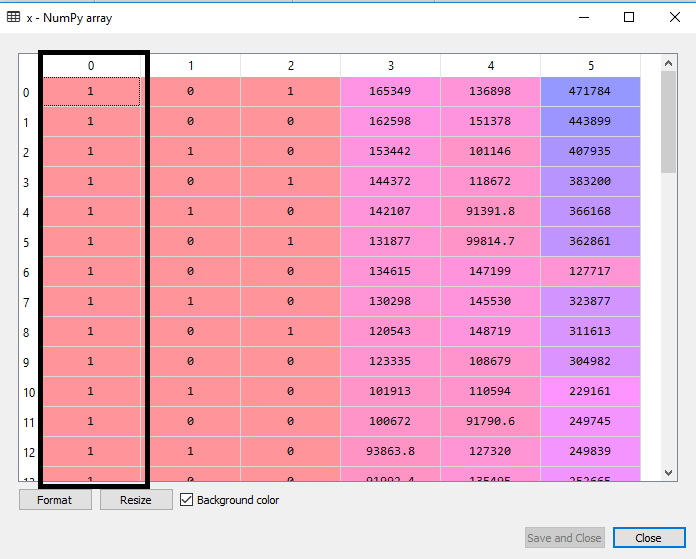
As we can see in the above output image, the first column is added successfully, which corresponds to the constant term of the MLR equation.
Step: 2:
- Now, we are actually going to apply a backward elimination process. Firstly we will create a new feature vector x_opt , which will only contain a set of independent features that are significantly affecting the dependent variable.
- Next, as per the Backward Elimination process, we need to choose a significant level(0.5), and then need to fit the model with all possible predictors. So for fitting the model, we will create a regressor_OLS object of new class OLS of statsmodels library. Then we will fit it by using the fit() method.
- Next we need p-value to compare with SL value, so for this we will use summary() method to get the summary table of all the values. Below is the code for it:
- x_opt=x [:, [0,1,2,3,4,5]]
- regressor_OLS=sm.OLS(endog = y, exog=x_opt).fit()
- regressor_OLS.summary()
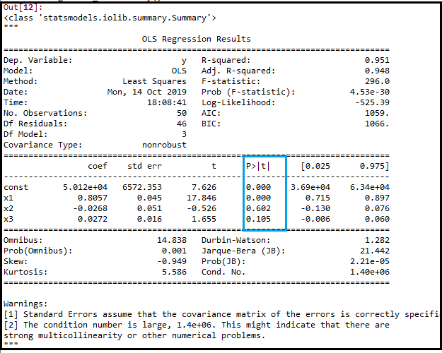
Output: By executing the above lines of code, we will get a summary table. Consider the below image:

In the above image, we can clearly see the p-values of all the variables. Here x1, x2 are dummy variables, x3 is R&D spend, x4 is Administration spend, and x5 is Marketing spend .
From the table, we will choose the highest p-value, which is for x1=0.953 Now, we have the highest p-value which is greater than the SL value, so will remove the x1 variable (dummy variable) from the table and will refit the model. Below is the code for it:
- x_opt=x[:, [0,2,3,4,5]]
- regressor_OLS=sm.OLS(endog = y, exog=x_opt).fit()
- regressor_OLS.summary()
Output:

As we can see in the output image, now five variables remain. In these variables, the highest p-value is 0.961. So we will remove it in the next iteration.
- Now the next highest value is 0.961 for x1 variable, which is another dummy variable. So we will remove it and refit the model. Below is the code for it:
- x_opt= x[:, [0,3,4,5]]
- regressor_OLS=sm.OLS(endog = y, exog=x_opt).fit()
- regressor_OLS.summary()
Output:
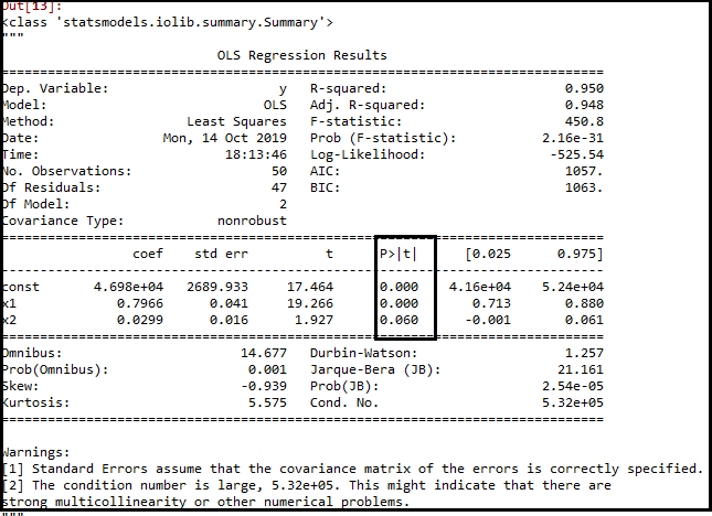
In the above output image, we can see the dummy variable(x2) has been removed. And the next highest value is .602, which is still greater than .5, so we need to remove it.
- Now we will remove the Admin spend which is having .602 p-value and again refit the model.
- x_opt=x[:, [0,3,5]]
- regressor_OLS=sm.OLS(endog = y, exog=x_opt).fit()
- regressor_OLS.summary()
Output:
As we can see in the above output image, the variable (Admin spend) has been removed. But still, there is one variable left, which is marketing spend as it has a high p-value (0.60) . So we need to remove it.
- Finally, we will remove one more variable, which has .60 p-value for marketing spend, which is more than a significant level.
Below is the code for it:
- x_opt=x[:, [0,3]]
- regressor_OLS=sm.OLS(endog = y, exog=x_opt).fit()
- regressor_OLS.summary()
Output:
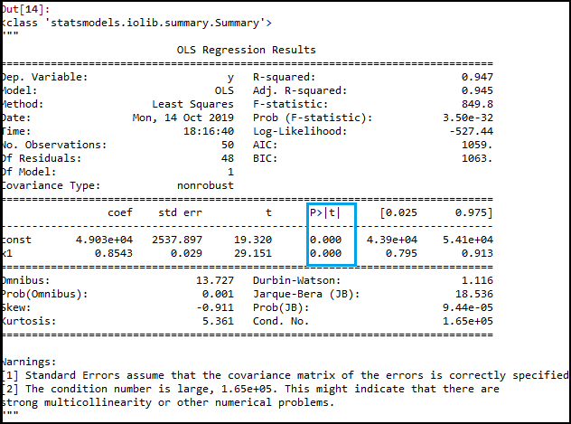
As we can see in the above output image, only two variables are left. So only the R&D independent variable is a significant variable for the prediction. So we can now predict efficiently using this variable.
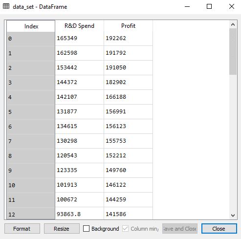
Estimating the performance:
In the previous topic, we have calculated the train and test score of the model when we have used all the features variables. Now we will check the score with only one feature variable (R&D spend). Our dataset now looks like:
Below is the code for Building Multiple Linear Regression model by only using R&D spend:
-
importing libraries
- import numpy as nm
- import matplotlib.pyplot as mtp
- import pandas as pd
- #importing datasets
- data_set= pd.read_csv(‘50_CompList1.csv’)
- #Extracting Independent and dependent Variable
- x_BE= data_set.iloc[:, :-1].values
- y_BE= data_set.iloc[:, 1].values
-
Splitting the dataset into training and test set.
- from sklearn.model_selection import train_test_split
- x_BE_train, x_BE_test, y_BE_train, y_BE_test= train_test_split(x_BE, y_BE, test_size= 0.2, random_state=0)
- #Fitting the MLR model to the training set:
- from sklearn.linear_model import LinearRegression
- regressor= LinearRegression()
- regressor.fit(nm.array(x_BE_train).reshape(-1,1), y_BE_train)
- #Predicting the Test set result;
- y_pred= regressor.predict(x_BE_test)
- #Cheking the score
- print('Train Score: ', regressor.score(x_BE_train, y_BE_train))
- print('Test Score: ', regressor.score(x_BE_test, y_BE_test))
Output:
After executing the above code, we will get the Training and test scores as:
Train Score: 0.9449589778363044 Test Score: 0.9464587607787219
As we can see, the training score is 94% accurate, and the test score is also 94% accurate. The difference between both scores is .00149 . This score is very much close to the previous score, i.e., 0.0154 , where we have included all the variables.
We got this result by using one independent variable (R&D spend) only instead of four variables. Hence, now, our model is simple and accurate.