Back-Propagation Algorithm

[swapneel-panda-419bc751 (Swapneel Panda)]

Back-Propagation Algorithm also called “backpropagation,” or simply “backprop,” is an algorithm for calculating the gradient of a loss function with respect to variables of a model.

• Back-Propagation: Algorithm for calculating the gradient of a loss function with respect to variables of a model.

You may recall from calculus that the first-order derivative of a function for a specific value of an input variable is the rate of change or curvature of the function for that input. When we have multiple input variables for a function, they form a vector and the vector of first-order derivatives (partial derivatives) is called the gradient (i.e. vector calculus).

• Gradient: Vector of partial derivatives of specific input values with respect to a target function.

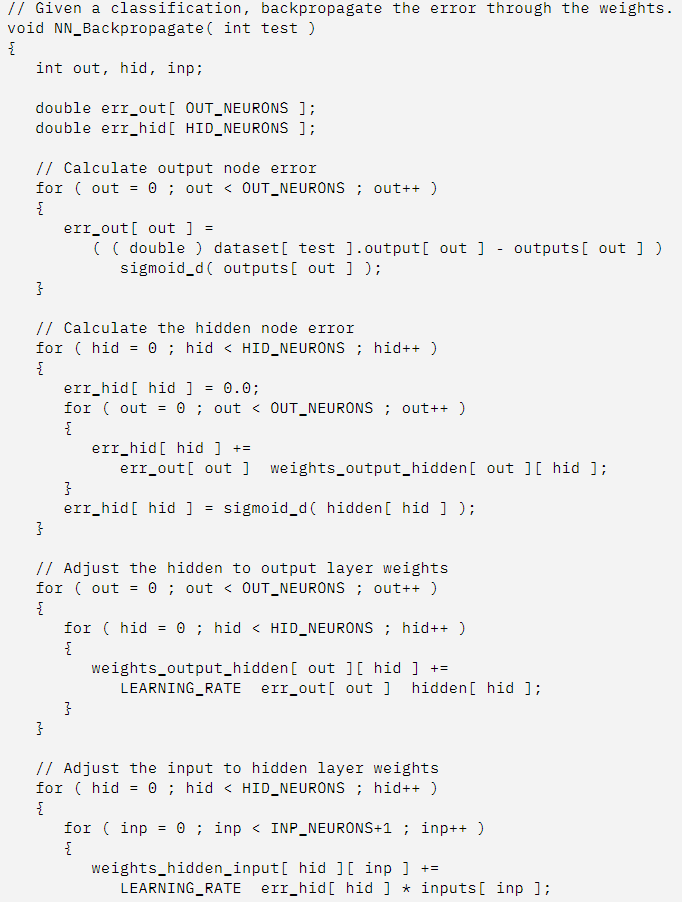
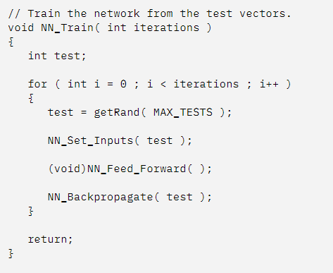
Back-propagation is used when training neural network models to calculate the gradient for each weight in the network model. The gradient is then used by an optimization algorithm to update the model weights.

The algorithm was developed explicitly for calculating the gradients of variables in graph structures working backward from the output of the graph toward the input of the graph, propagating the error in the predicted output that is used to calculate gradient for each variable.

The back-propagation algorithm, often simply called backprop, allows the information from the cost to then flow backwards through the network, in order to compute the gradient.

— Page 204, Deep Learning, 2016.

The loss function represents the error of the model or error function, the weights are the variables for the function, and the gradients of the error function with regard to the weights are therefore referred to as error gradients.

• Error Function: Loss function that is minimized when training a neural network.
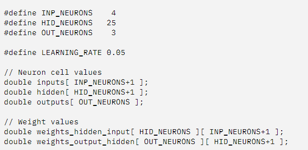
• Weights: Parameters of the network taken as input values to the loss function.
• Error Gradients: First-order derivatives of the loss function with regard to the parameters.

This gives the algorithm its name “back-propagation,” or sometimes “error back-propagation” or the “back-propagation of error.”

• Back-Propagation of Error: Comment on how gradients are calculated recursively backward through the network graph starting at the output layer.

The algorithm involves the recursive application of the chain rule from calculus (different from the chain rule from probability) that is used to calculate the derivative of a sub-function given the derivative of the parent function for which the derivative is known.

The chain rule of calculus […] is used to compute the derivatives of functions formed by composing other functions whose derivatives are known. Back-propagation is an algorithm that computes the chain rule, with a specific order of operations that is highly efficient.

— Page 205, Deep Learning, 2016.

• Chain Rule: Calculus formula for calculating the derivatives of functions using related functions whose derivatives are known.

There are other algorithms for calculating the chain rule, but the back-propagation algorithm is an efficient algorithm for the specific graph structured using a neural network.

It is fair to call the back-propagation algorithm a type of automatic differentiation algorithm and it belongs to a class of differentiation techniques called reverse accumulation.

The back-propagation algorithm described here is only one approach to automatic differentiation. It is a special case of a broader class of techniques called reverse mode accumulation.

— Page 222, Deep Learning, 2016.

Although Back-propagation was developed to train neural network models, both the back-propagation algorithm specifically and the chain-rule formula that it implements efficiently can be used more generally to calculate derivatives of functions.

[rohitkumar-singhvi-fe88d2d0 (Rohit Kumar Singhvi)]

Let’s have a look at a simple back-propagation implementation.

I use Fisher’s Iris flower data collection to train a primary network in this example.

This data collection contains four measures representing the length and width of flower petals and sepals in three iris flower species. The goal is to train the network to correctly categorize an iris using the four features that have been measured.

My variable definition is shown in the code below.

• With an input layer specifying my four features, a hidden layer containing 25 neurons, and an output layer representing a winner-takes-all representation of the three iris species, I define the size of my layers.
• The weights are represented by two multidimensional arrays that include biases, and the values of each neuron are defined by three collections (inputs, hidden, and outputs). There is also a low learning rate.

• The format of my training data set, which comprises individual training samples (of the four characteristics) with their species categorization, is shown in the following code example (into 1 of 3 output nodes). Because the complete data set has 150 samples, I’ve provided a condensed version here.

• The following code listing contains the code to run a network. This list can be divided into three sections. The first calculates the hidden layer neurons’ outputs using the input neurons.

• The hidden neurons are then used to calculate the outputs of the output layer neurons in the next part.

• The complete process of forwarding inputs over the network is called this (each layer using a sigmoidal activation function).

• The output neurons are iterated once the outputs have been calculated, and the most outstanding value is chosen in a winner-takes-all method. The solution is then returned as the output neuron.

Back-propagation is used to implement learning, as seen in the code example below.

This is accomplished in four steps.

• First, I calculate the output nodes’ error. Each is determined separately based on its inaccuracy (from the anticipated output) and the sigmoid function’s derivative.
• The buried layer neurons ’ error is determined based on their contribution to the output error.

The final two steps apply the mistakes to the output and hidden layers, using a learning rate to reduce the overall change and allow tuning over several rounds.

Gradient descent search is used in this procedure because the error in the neuron outputs is minimized (the gradient shows the most significant rate of increase of the error, so I move in the opposite direction of the slope).

The whole training process can be seen in the final section of this implementation.

I apply a random test case to the network, check the error, then back-propagate the error through the network’s weights using several iterations as my halting function.

The result of the back-propagation demonstration is seen in the sample output below.

A random sample of the data set is selected when the network is trained and tested against it.

The 10 test samples given below have been successfully categorized (the output is the output neuron index). The values in parenthesis are the desired output neuron values (the first is index 0, the second is index 1, and so on).