Python Implementation of Random Forest Algorithm

[vishrut-singhal]

we will implement the Random Forest Algorithm tree using Python. For this, we will use the same dataset “user_data.csv”, which we have used in previous classification models. By using the same dataset, we can compare the Random Forest classifier with other classification models such as Decision tree Classifier, KNN, SVM, Logistic Regression, etc.

Implementation Steps are given below:

• Data Pre-processing step
• Fitting the Random forest algorithm to the Training set
• Predicting the test result
• Test accuracy of the result (Creation of Confusion matrix)
• Visualizing the test set result.

1.Data Pre-Processing Step:

Below is the code for the pre-processing step:

1. importing libraries

2. import numpy as nm
3. import matplotlib.pyplot as mtp
4. import pandas as pd

• #importing datasets

5. data_set= pd.read_csv(‘user_data.csv’)

• #Extracting Independent and dependent Variable

6. x= data_set.iloc[:, [2,3]].values
7. y= data_set.iloc[:, 4].values

• Splitting the dataset into training and test set.

8. from sklearn.model_selection import train_test_split
9. x_train, x_test, y_train, y_test= train_test_split(x, y, test_size= 0.25, random_state=0)

• #feature Scaling

10. from sklearn.preprocessing import StandardScaler
11. st_x= StandardScaler()
12. x_train= st_x.fit_transform(x_train)
13. x_test= st_x.transform(x_test)

In the above code, we have pre-processed the data. Where we have loaded the dataset, which is given as:

2. Fitting the Random Forest algorithm to the training set:

Now we will fit the Random forest algorithm to the training set. To fit it, we will import the RandomForestClassifier class from the sklearn.ensemble library. The code is given below:

1. #Fitting Decision Tree classifier to the training set
2. from sklearn.ensemble import RandomForestClassifier
3. classifier= RandomForestClassifier(n_estimators= 10, criterion=“entropy”)
4. classifier.fit(x_train, y_train)

In the above code, the classifier object takes below parameters:

• n_estimators= The required number of trees in the Random Forest. The default value is 10. We can choose any number but need to take care of the overfitting issue.
• criterion= It is a function to analyze the accuracy of the split. Here we have taken “entropy” for the information gain.

Output:

RandomForestClassifier(bootstrap=True, class_weight=None, criterion=‘entropy’, max_depth=None, max_features=‘auto’, max_leaf_nodes=None, min_impurity_decrease=0.0, min_impurity_split=None, min_samples_leaf=1, min_samples_split=2, min_weight_fraction_leaf=0.0, n_estimators=10, n_jobs=None, oob_score=False, random_state=None, verbose=0, warm_start=False)

3. Predicting the Test Set result

Since our model is fitted to the training set, so now we can predict the test result. For prediction, we will create a new prediction vector y_pred. Below is the code for it:

1. #Predicting the test set result
2. y_pred= classifier.predict(x_test)

Output:

The prediction vector is given as:

By checking the above prediction vector and test set real vector, we can determine the incorrect predictions done by the classifier.

4. Creating the Confusion Matrix

Now we will create the confusion matrix to determine the correct and incorrect predictions. Below is the code for it:

1. #Creating the Confusion matrix
2. from sklearn.metrics import confusion_matrix
3. cm= confusion_matrix(y_test, y_pred)

Output:

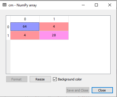
As we can see in the above matrix, there are 4+4= 8 incorrect predictions and 64+28= 92 correct predictions.

5. Visualizing the training Set result

Here we will visualize the training set result. To visualize the training set result we will plot a graph for the Random forest classifier. The classifier will predict yes or No for the users who have either Purchased or Not purchased the SUV car as we did in Logistic Regression. Below is the code for it:

1. from matplotlib.colors import ListedColormap
2. x_set, y_set = x_train, y_train
3. x1, x2 = nm.meshgrid(nm.arange(start = x_set[:, 0].min() - 1, stop = x_set[:, 0].max() + 1, step =0.01),
4. nm.arange(start = x_set[:, 1].min() - 1, stop = x_set[:, 1].max() + 1, step = 0.01))
5. mtp.contourf(x1, x2, classifier.predict(nm.array([x1.ravel(), x2.ravel()]).T).reshape(x1.shape),
6. alpha = 0.75, cmap = ListedColormap((‘purple’,‘green’ )))
7. mtp.xlim(x1.min(), x1.max())
8. mtp.ylim(x2.min(), x2.max())
9. for i, j in enumerate(nm.unique(y_set)):
10. mtp.scatter(x_set[y_set == j, 0], x_set[y_set == j, 1],
11. c = ListedColormap((‘purple’, ‘green’))(i), label = j)
12. mtp.title(‘Random Forest Algorithm (Training set)’)
13. mtp.xlabel(‘Age’)
14. mtp.ylabel(‘Estimated Salary’)
15. mtp.legend()
16. mtp.show()

Output:

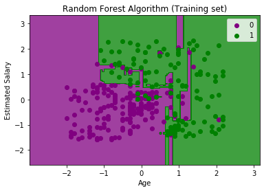
The above image is the visualization result for the Random Forest classifier working with the training set result. It is very much similar to the Decision tree classifier. Each data point corresponds to each user of the user_data, and the purple and green regions are the prediction regions. The purple region is classified for the users who did not purchase the SUV car, and the green region is for the users who purchased the SUV.

So, in the Random Forest classifier, we have taken 10 trees that have predicted Yes or NO for the Purchased variable. The classifier took the majority of the predictions and provided the result.

6. Visualizing the test set result

Now we will visualize the test set result. Below is the code for it:

1. #Visulaizing the test set result
2. from matplotlib.colors import ListedColormap
3. x_set, y_set = x_test, y_test
4. x1, x2 = nm.meshgrid(nm.arange(start = x_set[:, 0].min() - 1, stop = x_set[:, 0].max() + 1, step =0.01),
5. nm.arange(start = x_set[:, 1].min() - 1, stop = x_set[:, 1].max() + 1, step = 0.01))
6. mtp.contourf(x1, x2, classifier.predict(nm.array([x1.ravel(), x2.ravel()]).T).reshape(x1.shape),
7. alpha = 0.75, cmap = ListedColormap((‘purple’,‘green’ )))
8. mtp.xlim(x1.min(), x1.max())
9. mtp.ylim(x2.min(), x2.max())
10. for i, j in enumerate(nm.unique(y_set)):
11. mtp.scatter(x_set[y_set == j, 0], x_set[y_set == j, 1],
12. c = ListedColormap((‘purple’, ‘green’))(i), label = j)
13. mtp.title(‘Random Forest Algorithm(Test set)’)
14. mtp.xlabel(‘Age’)
15. mtp.ylabel(‘Estimated Salary’)
16. mtp.legend()
17. mtp.show()

Output:

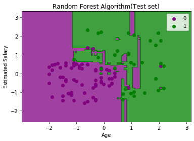
The above image is the visualization result for the test set. We can check that there is a minimum number of incorrect predictions (8) without the Overfitting issue. We will get different results by changing the number of trees in the classifier.