Python Implementation of K- Means Algorithm

[vishrut-singhal]

Before implementation, let’s understand what type of problem we will solve here. So, we have a dataset of Mall_Customers , which is the data of customers who visit the mall and spend there.

In the given dataset, we have Customer_Id, Gender, Age, Annual Income ($), and Spending Score (which is the calculated value of how much a customer has spent in the mall, the more the value, the more he has spent). From this dataset, we need to calculate some patterns, as it is an unsupervised method, so we don’t know what to calculate exactly.

The steps to be followed for the implementation are given below:

• Data Pre-processing
• Finding the optimal number of clusters using the elbow method
• Training the K-means algorithm on the training dataset
• Visualizing the clusters

Step-1: Data pre-processing Step

The first step will be the data pre-processing, as we did in our earlier topics of Regression and Classification. But for the clustering problem, it will be different from other models. Let’s discuss it:

• Importing Libraries
  As we did in previous topics, firstly, we will import the libraries for our model, which is part of data pre-processing. The code is given below:

1. importing libraries

2. import numpy as nm
3. import matplotlib.pyplot as mtp
4. import pandas as pd

In the above code, the numpy we have imported for the performing mathematics calculation, matplotlib is for plotting the graph, and pandas are for managing the dataset.

• Importing the Dataset:
  Next, we will import the dataset that we need to use. So here, we are using the Mall_Customer_data.csv dataset. It can be imported using the below code:

1. Importing the dataset

2. dataset = pd.read_csv(‘Mall_Customers_data.csv’)

By executing the above lines of code, we will get our dataset in the Spyder IDE. The dataset looks like the below image:

From the above dataset, we need to find some patterns in it.

• Extracting Independent Variables

Here we don’t need any dependent variable for data pre-processing step as it is a clustering problem, and we have no idea about what to determine. So we will just add a line of code for the matrix of features.

1. x = dataset.iloc[:, [3, 4]].values

As we can see, we are extracting only 3rd and 4th feature. It is because we need a 2d plot to visualize the model, and some features are not required, such as customer_id.

Step-2: Finding the optimal number of clusters using the elbow method

In the second step, we will try to find the optimal number of clusters for our clustering problem. So, as discussed above, here we are going to use the elbow method for this purpose.

As we know, the elbow method uses the WCSS concept to draw the plot by plotting WCSS values on the Y-axis and the number of clusters on the X-axis. So we are going to calculate the value for WCSS for different k values ranging from 1 to 10. Below is the code for it:

1. #finding optimal number of clusters using the elbow method
2. from sklearn.cluster import KMeans
3. wcss_list= [] #Initializing the list for the values of WCSS

• #Using for loop for iterations from 1 to 10.

4. for i in range(1, 11):
5. kmeans = KMeans(n_clusters=i, init=‘k-means++’, random_state= 42)
6. kmeans.fit(x)
7. wcss_list.append(kmeans.inertia_)
8. mtp.plot(range(1, 11), wcss_list)
9. mtp.title(‘The Elobw Method Graph’)
10. mtp.xlabel(‘Number of clusters(k)’)
11. mtp.ylabel(‘wcss_list’)
12. mtp.show()

As we can see in the above code, we have used the KMeans class of sklearn. cluster library to form the clusters.

Next, we have created the wcss_list variable to initialize an empty list, which is used to contain the value of wcss computed for different values of k ranging from 1 to 10.

After that, we have initialized the for loop for the iteration on a different value of k ranging from 1 to 10; since for loop in Python, exclude the outbound limit, so it is taken as 11 to include 10th value.

The rest part of the code is similar as we did in earlier topics, as we have fitted the model on a matrix of features and then plotted the graph between the number of clusters and WCSS.

Output: After executing the above code, we will get the below output:

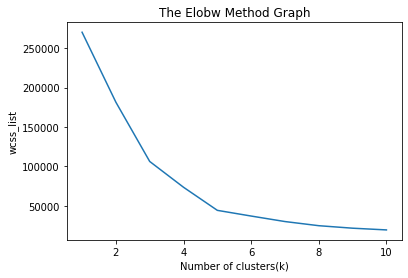
From the above plot, we can see the elbow point is at 5. So the number of clusters here will be 5.

Step- 3: Training the K-means algorithm on the training dataset

As we have got the number of clusters, so we can now train the model on the dataset.

To train the model, we will use the same two lines of code as we have used in the above section, but here instead of using i, we will use 5, as we know there are 5 clusters that need to be formed. The code is given below:

1. #training the K-means model on a dataset
2. kmeans = KMeans(n_clusters=5, init=‘k-means++’, random_state= 42)
3. y_predict= kmeans.fit_predict(x)

The first line is the same as above for creating the object of KMeans class.

In the second line of code, we have created the dependent variable y_predict to train the model.

By executing the above lines of code, we will get the y_predict variable. We can check it under the variable explorer option in the Spyder IDE. We can now compare the values of y_predict with our original dataset. Consider the below image:

From the above image, we can now relate that the CustomerID 1 belongs to a cluster

3(as index starts from 0, hence 2 will be considered as 3), and 2 belongs to cluster 4, and so on.

Step-4: Visualizing the Clusters

The last step is to visualize the clusters. As we have 5 clusters for our model, so we will visualize each cluster one by one.

To visualize the clusters will use scatter plot using mtp.scatter() function of matplotlib.

1. #visulaizing the clusters
2. mtp.scatter(x[y_predict == 0, 0], x[y_predict == 0, 1], s = 100, c = ‘blue’, label = ‘Cluster 1’) #for first cluster
3. mtp.scatter(x[y_predict == 1, 0], x[y_predict == 1, 1], s = 100, c = ‘green’, label = ‘Cluster 2’) #for second cluster
4. mtp.scatter(x[y_predict== 2, 0], x[y_predict == 2, 1], s = 100, c = ‘red’, label = ‘Cluster 3’) #for third cluster
5. mtp.scatter(x[y_predict == 3, 0], x[y_predict == 3, 1], s = 100, c = ‘cyan’, label = ‘Cluster 4’) #for fourth cluster
6. mtp.scatter(x[y_predict == 4, 0], x[y_predict == 4, 1], s = 100, c = ‘magenta’, label = ‘Cluster 5’) #for fifth cluster
7. mtp.scatter(kmeans.cluster_centers_[:, 0], kmeans.cluster_centers_[:, 1], s = 300, c = ‘yellow’, label = ‘Centroid’)
8. mtp.title(‘Clusters of customers’)
9. mtp.xlabel(‘Annual Income (k$)’)
10. mtp.ylabel(‘Spending Score (1-100)’)
11. mtp.legend()
12. mtp.show()

In above lines of code, we have written code for each clusters, ranging from 1 to 5. The first coordinate of the mtp.scatter, i.e., x[y_predict == 0, 0] containing the x value for the showing the matrix of features values, and the y_predict is ranging from 0 to 1.

Output:

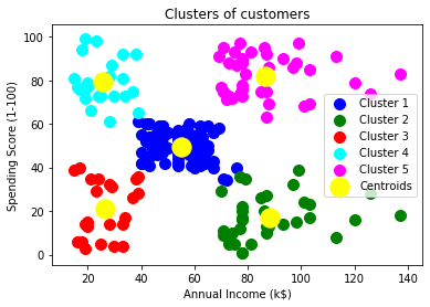
The output image is clearly showing the five different clusters with different colors. The clusters are formed between two parameters of the dataset; Annual income of customer and Spending. We can change the colors and labels as per the requirement or choice. We can also observe some points from the above patterns, which are given below:

• Cluster1 shows the customers with average salary and average spending so we can categorize these customers as
• Cluster2 shows the customer has a high income but low spending, so we can categorize them as careful .
• Cluster3 shows the low income and also low spending so they can be categorized as sensible.
• Cluster4 shows the customers with low income with very high spending so they can be categorized as careless .
• Cluster5 shows the customers with high income and high spending so they can be categorized as target, and these customers can be the most profitable customers for the mall owner.