Logistic regression in R

[vishrut-singhal]

R-Logistic Regression

In the logistic regression, a regression curve, y = f (x), is fitted. In the regression curve equation, y is a categorical variable. This Regression Model is used for predicting that y has given a set of predictors x. Therefore, predictors can be categorical, continuous, or a mixture of both.

The logistic regression is a classification algorithm that falls under nonlinear regression. This model is used to predict a given binary result (1/0, yes/no, true/false) as a set of independent variables. Furthermore, it helps to represent categorical/binary outcomes using dummy variables.

Logistic regression is a regression model in which the response variable has categorical values such as true/false or 0/1. Therefore, we can measure the probability of the binary response.

There is the following mathematical equation for the logistic regression:

y=1/(1+e^-(b0+b1 x1+b2 x2+⋯))

In the above equation, y is a response variable, x is the predictor variable, and b0 and b1, b2,…bn are the coefficients, which is numeric constants. We use the glm() function to create the regression model.

There is the following syntax of the glm() function.

glm(formula, data, family)

Here,

S.No	Parameter	Description
1.	formula	It is a symbol which represents the relationship b/w the variables.
2.	data	It is the dataset giving the values of the variables.
3.	family	An R object which specifies the details of the model, and its value is binomial for logistic regression.

Building Logistic Regression

The in-built data set “mtcars” describes various models of the car with their different engine specifications. In the “mtcars” data set, the transmission mode is described by the column “am”, which is a binary value (0 or 1). We can construct a logistic regression model between column “am” and three other columns - hp, wt, and cyl.

Let’s see an example to understand how the glm function is used to create logistic regression and how we can use the summary function to find a summary for the analysis.

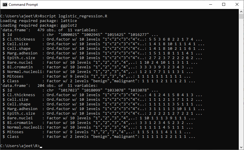
In our example, we will use the dataset “BreastCancer” available in the R environment. To use it, we first need to install “mlbench” and “caret” packages.

Example

#Loading library  
library(mlbench)  
#Using BreastCancer dataset  
data(BreastCancer, package = "mlbench")  
breast_canc = BreastCancer[complete.cases(BreastCancer),]  
#Displaying the information related to dataset with the str() function.  
str(breast_canc)  

Output:

We now divide our data into training and test sets with training sets containing 70% data and test sets including the remaining percentages.

#Dividing dataset into training and test dataset.  
set.seed(100)  
#Creating partitioning.  
Training_Ratio <- createDataPartition(b_canc$Class, p=0.7, list = F)  
#Creating training data.  
Training_Data <- b_canc[Training_Ratio, ]  
str(Training_Data)  
#Creating test data.  
Test_Data <- b_canc[-Training_Ratio, ]  
str(Test_Data)  

Output:

Now, we construct the logistic regression function with the help of glm() function. We pass the formula Class~Cell.shape as the first parameter and specifying the attribute family as " binomial " and use Training_data as the third parameter.

Example

#Creating Regression Model  
glm(Class ~ Cell.shape, family="binomial", data = Training_Data)  

Output:

Now, use the summary function for analysis.

#Creating Regression Model  
model<-glm(Class ~ Cell.shape, family="binomial", data = Training_Data)  
#Using summary function  
print(summary(model)) 

Output: